3 Índices de centralidad
3.1 Insumos y paquetes
Seguimos trabajando con los mismos shapefiles de la sección anterior: habitat_nodes y paisaje.
#> Cargando paquete requerido: igraph
#>
#> Adjuntando el paquete: 'igraph'
#> The following objects are masked from 'package:stats':
#>
#>     decompose, spectrum
#> The following object is masked from 'package:base':
#>
#>     union
#> Cargando paquete requerido: cppRouting
#> Linking to GEOS 3.13.0, GDAL 3.10.1, PROJ 9.5.1;
#> sf_use_s2() is TRUE
#> [1] 404
ggplot() +
  geom_sf(data = paisaje, aes(color = "Study area"), fill = NA, color = "black") +
  geom_sf(data = habitat_nodes, aes(color = "Parches"), fill = "forestgreen", linewidth = 0.5) +
  scale_color_manual(name = "", values = "black")+
  theme_minimal() +
  theme(axis.title.x = element_blank(),
        axis.title.y = element_blank())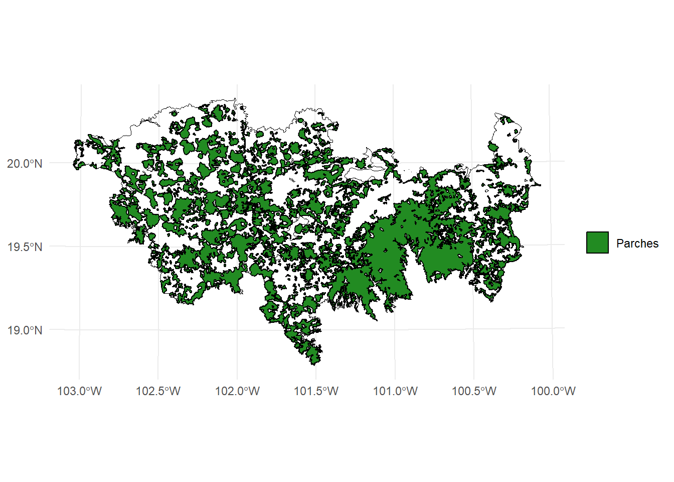
En caso de necesitar abrir otro vector (e.g., .shp, .gpkg) necesitan usar la fución read_sf() del paquete sf, la función shapefile() del paquete raster, o la funcion vect() del paquete terra.
Para abrirlo solo necesitan colocar la dirección de su archivo, el nombre y la extensión, ejemplo:
vegetation_patches <- sf::read_sf("D:/Datos/vegetation_patches.shp")vegetation_patches <- raster::shapefile("D:/Datos/vegetation_patches.shp")vegetation_patches <- terra::vect("D:/Datos/vegetation_patches.shp")
3.2 MK_RMCentrality()
La función MK_RMCentrality() calcula medidas radiales (es decir, grado, fuerza, centralidad de vectores propios y centralidad de proximidad) y mediales (es decir, centralidad de interrelación, pertenencia a nodos y modularidad) de la centralidad de nodos para identificar, por ejemplo, stepping stones.
Las medidas o índices que estima son los siguientes:
3.2.1 1. Centralidad de Grado (degree)
Cuántas conexiones directas tiene un nodo.
- Es como contar cuántos parches de hábitat o áreas protegidas están conectados con cada parche.
- Más conexiones = mayor grado = más centralidad.
3.2.2 2. Fuerza (strength) (para redes ponderadas)
Como el grado, pero suma los pesos (o probabilidades) de los enlaces.
- En lugar de solo contar conexiones, se suman qué tan fuertes o probables son (por ejemplo, probabilidad de dispersión).
- Un nodo con pocas pero fuertes conexiones puede ser más central que uno con muchas pero débiles.
3.2.3 3. Centralidad de Vector Propio (eigen)
Mide cuán conectado está un nodo con otros nodos importantes para la conectividad.
- Un nodo es importante si está conectado a otros nodos que también lo son.
- Útil para detectar “nodos influyentes” en la red.
3.2.4 4. Centralidad de Cercanía (close)
Qué tan cerca está un nodo de todos los demás.
- Se calcula como el inverso de la suma de distancias a todos los demás nodos.
- Los nodos con alta cercanía pueden difundir o recibir flujo rápidamente.
3.2.6 Detección de Comunidades (¿Quién pertenece al mismo grupo?)
3.2.7 La función (no correr)
MK_RMCentrality(
  nodes,
  distance = list(type = "centroid"),
  distance_thresholds = NULL,
  binary = TRUE,
  probability = NULL,
  rasterparallel = FALSE,
  write = NULL,
  intern = TRUE
)
3.2.8 Descripción de los argumentos de la función
| Argumento | Tipo | Descripción |
|---|---|---|
nodes |
objeto | Objeto que representa los nodos o fragmentos de hábitat. Puede ser un data.frame, objeto espacial vectorial (sf, SpatVector, etc.) o raster (RasterLayer, SpatRaster). Debe estar en un sistema de coordenadas proyectadas. En rasters, los valores deben ser enteros (ID de los nodos) y los no hábitat como NA. |
distance |
matriz o lista | Matriz cuadrada con las distancias entre nodos o una lista con los parámetros para calcularlas. Puede incluir tipo ("centroid", "edge", "least-cost", "commute-time") y resistencia. |
distance_thresholds |
numérico | Distancia de dispersión (en metros) de la especie. Si es NULL, se calcula como la mediana entre nodos. También se puede estimar con la función dispersal_distance. |
binary |
lógico | Si es TRUE, se calcula conectividad binaria: nodos conectados (1) o no conectados (0) según el umbral de distancia. No usa probability. |
probability |
numérico | Probabilidad de conexión asociada al umbral de distancia. Por ejemplo, 0.5 para distancias medianas, 0.05 para distancias máximas. Por defecto es 0.5 si es NULL. |
rasterparallel |
lógico | Si nodes es un raster, permite asignar las métricas calculadas al raster de nodos. Útil cuando la resolución es menor a 100 m². |
write |
texto | Ruta y prefijo para guardar los resultados (sf). Ejemplo: "C:/ejemplo". |
intern |
lógico | Muestra el progreso del proceso. Por defecto TRUE. Puede no llegar al 100% si el cálculo es muy rápido. |
3.3 Ejemplo 1
library(Makurhini)
library(sf)
data("habitat_nodes", package = "Makurhini")
nrow(habitat_nodes) # Number of patches
#> [1] 404
#Two distance threshold,
centrality_test <- MK_RMCentrality(nodes = habitat_nodes,
                                distance = list(type = "centroid"),
                                 distance_thresholds = 10000,
                                 probability = 0.5,
                                 write = NULL)
#> Done!
centrality_test
#> Simple feature collection with 404 features and 8 fields
#> Geometry type: POLYGON
#> Dimension:     XY
#> Bounding box:  xmin: -108954 ymin: 2025032 xmax: 202330.2 ymax: 2198936
#> Projected CRS: NAD_1927_Albers
#> First 10 features:
#>    Id strength        eigen      close  BWC cluster memb.rw
#> 1   1 30228524 0.0010435836 0.03840356    0       1       6
#> 2   2 21600031 0.0006195356 0.03995935    1       1       6
#> 3   3 29320545 0.0009026418 0.03831019    0       1       6
#> 4   4 16499522 0.0005867564 0.04187906   23       1       6
#> 5   5 26068911 0.0011987437 0.04240465    0       1       6
#> 6   6 12737692 0.0005630043 0.04627714   17       1       6
#> 7   7 12497243 0.0005499038 0.04634291   15       1       6
#> 8   8 13198398 0.0005859873 0.04607765    0       1       6
#> 9   9 22276433 0.0010276194 0.04296412  567       1       6
#> 10 10 12804425 0.0004306005 0.04405417 1063       1       6
#>    memb.louvain                       geometry
#> 1             1 POLYGON ((54911.05 2035815,...
#> 2             1 POLYGON ((44591.28 2042209,...
#> 3             1 POLYGON ((46491.11 2042467,...
#> 4             1 POLYGON ((54944.49 2048163,...
#> 5             2 POLYGON ((80094.28 2064140,...
#> 6             2 POLYGON ((69205.24 2066394,...
#> 7             2 POLYGON ((68554.2 2066632, ...
#> 8             2 POLYGON ((69995.53 2066880,...
#> 9             2 POLYGON ((79368.68 2067324,...
#> 10            1 POLYGON ((23378.32 2067554,...
Exploremos otra forma de hacer el plot usando intervalos
install.packages("ClassInt", dependencies = TRUE)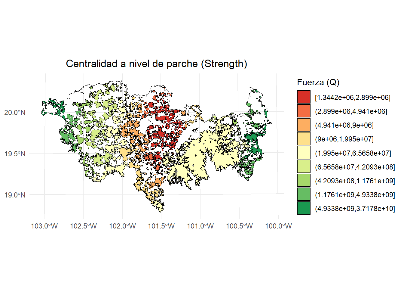
install.packages("dplyr", dependencies = TRUE)- Strength:
library(classInt)
library(dplyr)
#>
#> Adjuntando el paquete: 'dplyr'
#> The following objects are masked from 'package:igraph':
#>
#>     as_data_frame, groups, union
#> The following objects are masked from 'package:stats':
#>
#>     filter, lag
#> The following objects are masked from 'package:base':
#>
#>     intersect, setdiff, setequal, union

# Calcular los intervalos de Jenks para strength
breaks <- classInt::classIntervals(centrality_test$strength, n = 9, style = "quantile")

# Crear una nueva variable categórica con los intervalos
centrality_test <- centrality_test %>%
  mutate(strength_q = cut(strength,
                              breaks = breaks$brks,
                              include.lowest = TRUE,
                              dig.lab = 5))

# Graficar en ggplot2 usando las clases Jenks
ggplot() +
  geom_sf(data = paisaje, fill = NA, color = "black") +
  geom_sf(data = centrality_test, aes(fill = strength_q), color = "black", size = 0.1) +
  scale_fill_brewer(palette = "RdYlGn", direction = 1, name = "Fuerza (Q)") +
  theme_minimal() +
  labs(
    title = "Centralidad a nivel de parche (Strength)",
    fill = "Strength\n(Jenks)"
  ) +
  theme(
    legend.position = "right",
    plot.title = element_text(hjust = 0.5)
  )
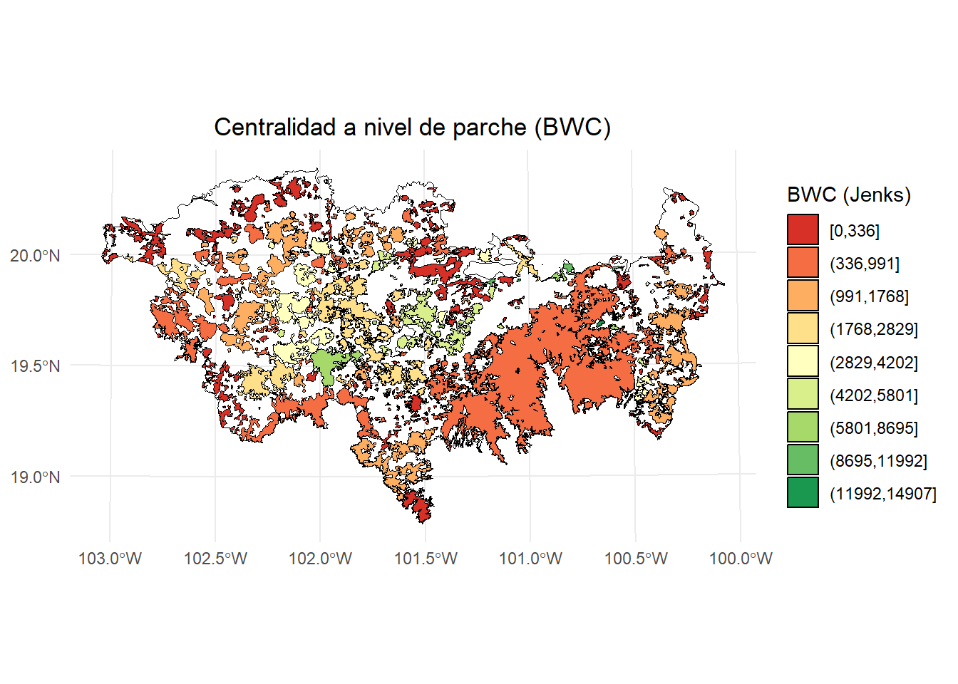
- BWC:
breaks <- classInt::classIntervals(centrality_test$BWC, n = 9, style = "jenks")
centrality_test <- centrality_test %>%
  mutate(BWC_jenks = cut(BWC,
                              breaks = breaks$brks,
                              include.lowest = TRUE,
                              dig.lab = 5))
ggplot() +
  geom_sf(data = paisaje, fill = NA, color = "black") +
  geom_sf(data = centrality_test, aes(fill = BWC_jenks), color = "black", size = 0.1) +
  scale_fill_brewer(palette = "RdYlGn", direction = 1, name = "BWC (Jenks)") +
  theme_minimal() +
  labs(
    title = "Centralidad a nivel de parche (BWC)",
    fill = "BWC\n(Jenks)"
  ) +
  theme(
    legend.position = "right",
    plot.title = element_text(hjust = 0.5)
  )
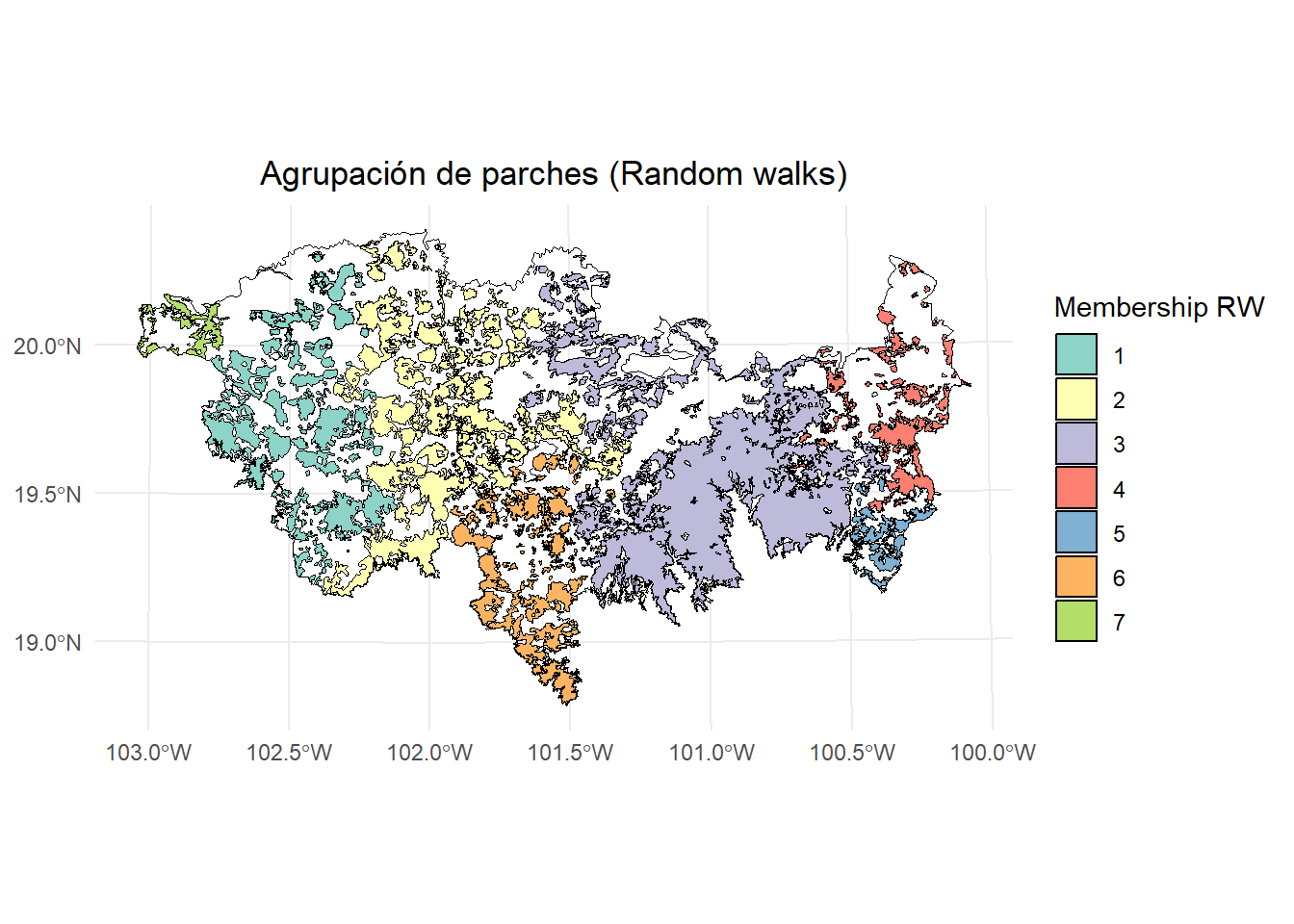
- Membresía por random walk:
ggplot() +
  geom_sf(data = paisaje, fill = NA, color = "black") +
  geom_sf(data = centrality_test, aes(fill = as.factor(memb.rw)), color = "black", size = 0.1) +
  scale_fill_brewer(
    palette = "Set3",
    name = "Membership RW"
  ) +
  theme_minimal() +
  labs(
    title = "Agrupación de parches (Random walks)",
    fill = "Membership RW"
  ) +
  theme(
    legend.position = "right",
    plot.title = element_text(hjust = 0.5)
  )
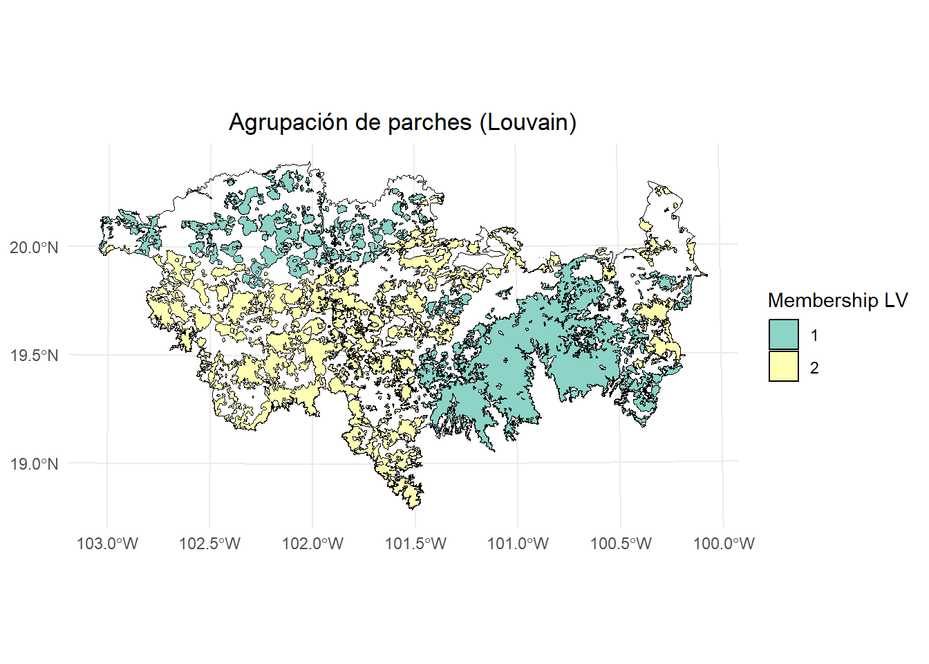
- Membresía por Louvain:
ggplot() +
  geom_sf(data = paisaje, fill = NA, color = "black") +
  geom_sf(data = centrality_test, aes(fill = as.factor(memb.louvain)), color = "black", size = 0.1) +
  scale_fill_brewer(
    palette = "Set3",
    name = "Membership LV"
  ) +
  theme_minimal() +
  labs(
    title = "Agrupación de parches (Louvain)",
    fill = "Membership LV"
  ) +
  theme(
    legend.position = "right",
    plot.title = element_text(hjust = 0.5)
  )
3.4 Ejemplo 2
Usando más de un umbral de distancia
centrality_test <- MK_RMCentrality(nodes = habitat_nodes,
                                distance = list(type = "centroid"),
                                 distance_thresholds = c(10000, 100000),
                                 probability = 0.5,
                                 write = NULL)
#> Done!
centrality_test
#> $d10000
#> Simple feature collection with 404 features and 8 fields
#> Geometry type: POLYGON
#> Dimension:     XY
#> Bounding box:  xmin: -108954 ymin: 2025032 xmax: 202330.2 ymax: 2198936
#> Projected CRS: NAD_1927_Albers
#> First 10 features:
#>    Id strength        eigen      close  BWC cluster memb.rw
#> 1   1 30228524 0.0010435836 0.03840356    0       1       6
#> 2   2 21600031 0.0006195356 0.03995935    1       1       6
#> 3   3 29320545 0.0009026418 0.03831019    0       1       6
#> 4   4 16499522 0.0005867564 0.04187906   23       1       6
#> 5   5 26068911 0.0011987437 0.04240465    0       1       6
#> 6   6 12737692 0.0005630043 0.04627714   17       1       6
#> 7   7 12497243 0.0005499038 0.04634291   15       1       6
#> 8   8 13198398 0.0005859873 0.04607765    0       1       6
#> 9   9 22276433 0.0010276194 0.04296412  567       1       6
#> 10 10 12804425 0.0004306005 0.04405417 1063       1       6
#>    memb.louvain                       geometry
#> 1             1 POLYGON ((54911.05 2035815,...
#> 2             2 POLYGON ((44591.28 2042209,...
#> 3             2 POLYGON ((46491.11 2042467,...
#> 4             1 POLYGON ((54944.49 2048163,...
#> 5             1 POLYGON ((80094.28 2064140,...
#> 6             1 POLYGON ((69205.24 2066394,...
#> 7             1 POLYGON ((68554.2 2066632, ...
#> 8             1 POLYGON ((69995.53 2066880,...
#> 9             1 POLYGON ((79368.68 2067324,...
#> 10            2 POLYGON ((23378.32 2067554,...
#>
#> $`d1e+05`
#> Simple feature collection with 404 features and 8 fields
#> Geometry type: POLYGON
#> Dimension:     XY
#> Bounding box:  xmin: -108954 ymin: 2025032 xmax: 202330.2 ymax: 2198936
#> Projected CRS: NAD_1927_Albers
#> First 10 features:
#>    Id strength     eigen     close BWC cluster memb.rw
#> 1   1 958.4815 0.6679253 0.4207380   0       1       1
#> 2   2 925.0415 0.6471542 0.4356561   0       1       1
#> 3   3 960.2533 0.6700437 0.4197704   0       1       1
#> 4   4 896.6891 0.6266304 0.4494531   0       1       1
#> 5   5 871.2094 0.6057986 0.4632174   0       1       1
#> 6   6 836.4790 0.5842254 0.4818295   0       1       1
#> 7   7 836.5028 0.5843345 0.4818097   0       1       1
#> 8   8 837.6158 0.5848721 0.4811889   0       1       1
#> 9   9 858.0974 0.5971238 0.4701554   0       1       1
#> 10 10 874.7611 0.6125436 0.4606972   0       1       1
#>    memb.louvain                       geometry
#> 1             1 POLYGON ((54911.05 2035815,...
#> 2             1 POLYGON ((44591.28 2042209,...
#> 3             1 POLYGON ((46491.11 2042467,...
#> 4             1 POLYGON ((54944.49 2048163,...
#> 5             1 POLYGON ((80094.28 2064140,...
#> 6             1 POLYGON ((69205.24 2066394,...
#> 7             1 POLYGON ((68554.2 2066632, ...
#> 8             1 POLYGON ((69995.53 2066880,...
#> 9             1 POLYGON ((79368.68 2067324,...
#> 10            1 POLYGON ((23378.32 2067554,...
10 km:
plot(centrality_test$d10000["BWC"], breaks = "quantile")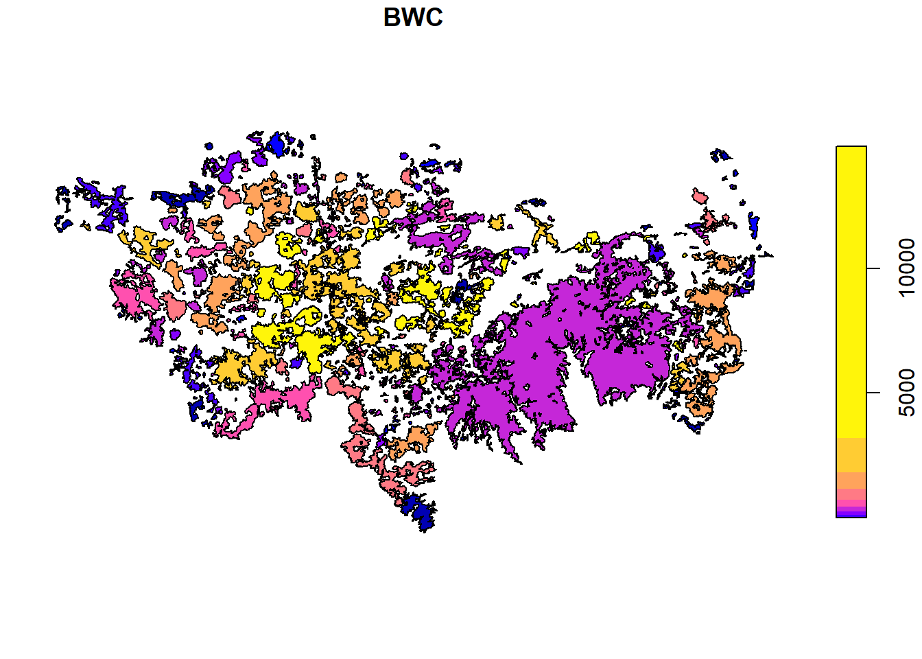
100 km:
plot(centrality_test$`d1e+05`["BWC"], breaks = "quantile")