5 índice integral de conectividad y Probabilidad de conectividad
5.1 Insumos y paquetes
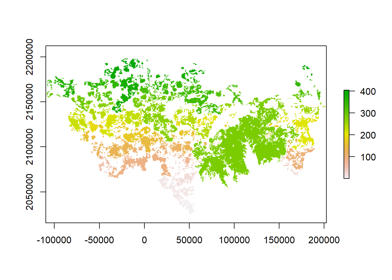
Seguimos trabajando con los mismos shapefiles de la sección anterior: habitat_nodes y paisaje.
#> Linking to GEOS 3.13.0, GDAL 3.10.1, PROJ 9.5.1;
#> sf_use_s2() is TRUE
#> [1] 404
ggplot() +
  geom_sf(data = paisaje, aes(color = "Study area"), fill = NA, color = "black") +
  geom_sf(data = habitat_nodes, aes(color = "Parches"), fill = "forestgreen", linewidth = 0.5) +
  scale_color_manual(name = "", values = "black")+
  theme_minimal() +
  theme(axis.title.x = element_blank(),
        axis.title.y = element_blank())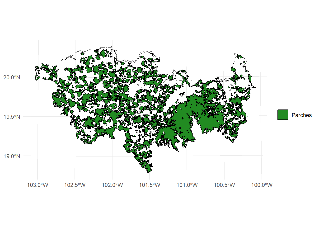
5.2 MK_dPCIIC()
Esta función calcula tanto la conectividad global del paisaje como la importancia (contribución) de cada nodo (o parche de hábitat) para mantener la conectividad del paisaje. Utiliza los índices PC e IIC bajo uno o varios umbrales de distancia.
5.2.1 La función (no correr)
MK_dPCIIC(
  nodes,
  attribute = NULL,
  weighted = FALSE,
  LA = NULL,
  area_unit = "m2",
  restoration = NULL,
  onlyrestor = FALSE,
  distance = list(type = "centroid", resistance = NULL),
  metric = c("IIC", "PC"),
  probability = NULL,
  distance_thresholds = NULL,
  threshold = NULL,
  overall = FALSE,
  onlyoverall = FALSE,
  parallel = NULL,
  parallel_mode = 1,
  write = NULL,
  id_sel = NULL,
  intern = TRUE
)
5.2.2 Descripción de los argumentos de la función
| Argumento | Descripción |
|---|---|
nodes |
Objeto que contiene la información de los nodos (e.g., fragmentos de hábitat). Puede ser un data.frame (mínimo dos columnas: ID y atributo), un objeto espacial vectorial (sf, SpatVector) o un raster con valores enteros que representen los ID de cada nodo. Debe estar en un sistema de coordenadas proyectadas. |
attribute |
Nombre de la columna o vector numérico con el atributo de los nodos. Si es NULL, se utiliza el área como atributo. Si nodes es raster, debe ser un vector numérico de igual longitud al número de nodos. |
weighted |
Lógico. Si TRUE y nodes es raster, el atributo será ponderado por el área de cada nodo. |
LA |
Valor numérico (opcional). Atributo máximo del paisaje. Por ejemplo, el área total si el atributo es área. Se usa para calcular la conectividad global, no afecta la importancia relativa de nodos. |
area_unit |
Unidad de área (opcional, por defecto "m2"). Puede ser "m2", "km2", "cm2" o "ha". |
restoration |
Vector o nombre de columna que indica si cada nodo es existente (1) o propuesto para restauración (0). Si es NULL, se considera que todos los nodos existen. |
onlyrestor |
Lógico. Si TRUE, solo se calcularán métricas relacionadas con restauración. |
distance |
Matriz o lista con parámetros para calcular distancia entre nodos. Puede ser matriz de distancias o una lista con parámetros como type (i.e., "centroid", "edge",``"least-cost",``"commute-time") y resistance (raster de resistencia). |
metric |
Métrica de conectividad a usar: "PC" (probabilidad de conectividad) o "IIC" (índice integral de conectividad). |
probability |
Valor numérico que representa la probabilidad asociada a la distancia umbral (e.g., 0.5 si es la mediana de dispersión). Solo se usa con la métrica "PC". |
distance_thresholds |
Distancia(s) de dispersión en metros. Si es NULL, se estima como la mediana de dispersión entre nodos. Puede usarse la función dispersal_distance. |
threshold |
Distancia máxima entre pares de nodos a considerar. Mejora eficiencia al eliminar pares lejanos. |
overall |
Lógico. Si TRUE, se calcula el índice de conectividad del paisaje completo (EC). El resultado será una lista. |
onlyoverall |
Lógico. Si TRUE, solo se calcularán métricas globales del paisaje. |
parallel |
Número de núcleos a usar en paralelización para estimar índices. Útil con más de 1000 nodos. |
parallel_mode |
Modo de paralelización: 1 (por defecto, recomendado < 1000 nodos) o 2 (recomendado > 1000 nodos). |
write |
Ruta y prefijo para guardar los resultados (e.g., "C:/ejemplo/test_PC_"). Se guardan archivos de importancia de nodos y conectividad general si overall = TRUE. |
id_sel |
Uso interno. No debe usarse por el usuario. |
intern |
Lógico. Muestra el progreso del proceso (TRUE por defecto). |
5.4 Ejemplo 1. Distancia euclidiana
- Sin usar LA
- sin usar attribute
- 10 km de mediana de dispersión
- Unidad de área en ha
- Solo índice para todo el paisaje
IIC <- MK_dPCIIC(nodes = habitat_nodes,
                attribute = NULL,
                area_unit = "ha",
                distance = list(type = "centroid"),
                LA = NULL,
                onlyoverall = TRUE,
                metric = "IIC",
                distance_thresholds = 10000,
                intern = TRUE) #10 km
#> Estimating IIC index. This may take several minutes depending on the number of nodes
#>
  |
  |                                                  |   0%
#>
#> Done!
IIC
#>     Index        Value
#> 1  IICnum 1.434310e+12
#> 2 EC(IIC) 1.197627e+06
5.5 Ejemplo 2. Distancia euclidiana
- sin usar attribute
- 10 km de mediana de dispersión
- Unidad de área en ha
- Solo índice para todo el paisaje
area_paisaje <- st_area(paisaje)
area_paisaje <- unit_convert(area_paisaje, "m2", "ha")

IIC <- MK_dPCIIC(nodes = habitat_nodes,
                attribute = NULL,
                area_unit = "ha",
                distance = list(type = "centroid"),
                LA = area_paisaje,
                onlyoverall = TRUE,
                metric = "IIC",
                distance_thresholds = 10000,
                intern = TRUE) #10 km
#> Estimating IIC index. This may take several minutes depending on the number of nodes
#>
  |
  |                                                  |   0%
#>
#> Done!
IIC
#>     Index        Value
#> 1  IICnum 1.434310e+12
#> 2 EC(IIC) 1.197627e+06
#> 3     IIC 1.881017e-01
5.6 Ejemplo 3. Distancia euclidiana
- sin usar attribute
- 10 km de mediana de dispersión
- Unidad de área en ha
- Solo índice para todo el paisaje
area_paisaje <- st_area(paisaje)
area_paisaje <- unit_convert(area_paisaje, "m2", "ha")

IIC <- MK_dPCIIC(nodes = habitat_nodes,
                attribute = NULL,
                area_unit = "ha",
                distance = list(type = "edge"),
                LA = area_paisaje,
                onlyoverall = TRUE,
                metric = "IIC",
                distance_thresholds = 10000,
                intern = TRUE) #10 km
#> Estimating IIC index. This may take several minutes depending on the number of nodes
#>
  |
  |                                                  |   0%
#>
#> Done!
IIC
#>     Index        Value
#> 1  IICnum 5.700691e+11
#> 2 EC(IIC) 7.550292e+05
#> 3     IIC 7.476136e-02
area_paisaje <- st_area(paisaje)
area_paisaje <- unit_convert(area_paisaje, "m2", "ha")
IIC <- MK_dPCIIC(nodes = habitat_nodes,
attribute = NULL,
area_unit = "ha",
distance = list(type = "edge", keep = 0.1),
LA = area_paisaje,
onlyoverall = TRUE,
metric = "IIC",
distance_thresholds = 10000,
intern = TRUE) #10 km
#> Estimating IIC index. This may take several minutes depending on the number of nodes
#>
|
| | 0%
#>
#> Done!
IIC
#> Index Value
#> 1 IICnum 5.693868e+11
#> 2 EC(IIC) 7.545772e+05
#> 3 IIC 7.467188e-025.7 Ejemplo 4. Distancia euclidiana: fracciones
- sin usar attribute
- 10 km de mediana de dispersión
- Unidad de área en ha
area_paisaje <- st_area(paisaje)
area_paisaje <- unit_convert(area_paisaje, "m2", "ha")

IIC <- MK_dPCIIC(nodes = habitat_nodes,
                attribute = NULL,
                area_unit = "ha",
                distance = list(type = "edge", keep = 0.1),
                LA = area_paisaje,
                onlyoverall = FALSE,
                metric = "IIC",
                distance_thresholds = 10000,
                intern = TRUE) #10 km
#> Estimating IIC index. This may take several minutes depending on the number of nodes
#>
  |
  |                                                  |   0%
#>  ■■■■■■■■■■■■■                     39% |  ETA:  3s
#>
#> Done!
IIC
#> Simple feature collection with 404 features and 5 fields
#> Geometry type: POLYGON
#> Dimension:     XY
#> Bounding box:  xmin: -108954 ymin: 2025032 xmax: 202330.2 ymax: 2198936
#> Projected CRS: NAD_1927_Albers
#> First 10 features:
#>    Id      dIIC dIICintra  dIICflux dIICconnector
#> 1   1 0.0067065 0.0000013 0.0067052   0.000000000
#> 2   2 0.0210320 0.0000085 0.0210235   0.000000000
#> 3   3 1.0591462 0.0213281 1.0312790   0.006539041
#> 4   4 0.0115557 0.0000026 0.0115531   0.000000000
#> 5   5 0.0254291 0.0000060 0.0254231   0.000000000
#> 6   6 0.0036214 0.0000001 0.0036212   0.000000000
#> 7   7 0.0059875 0.0000003 0.0059872   0.000000000
#> 8   8 0.0079222 0.0000006 0.0079216   0.000000000
#> 9   9 0.0280103 0.0000073 0.0280030   0.000000000
#> 10 10 4.5575494 0.1522233 3.3954709   1.009855242
#>                          geometry
#> 1  POLYGON ((54911.05 2035815,...
#> 2  POLYGON ((44591.28 2042209,...
#> 3  POLYGON ((46491.11 2042467,...
#> 4  POLYGON ((54944.49 2048163,...
#> 5  POLYGON ((80094.28 2064140,...
#> 6  POLYGON ((69205.24 2066394,...
#> 7  POLYGON ((68554.2 2066632, ...
#> 8  POLYGON ((69995.53 2066880,...
#> 9  POLYGON ((79368.68 2067324,...
#> 10 POLYGON ((23378.32 2067554,...
Exploremos un plot usando intervalos:
- dIIC
library(classInt)
library(dplyr)
#>
#> Adjuntando el paquete: 'dplyr'
#> The following objects are masked from 'package:igraph':
#>
#>     as_data_frame, groups, union
#> The following objects are masked from 'package:stats':
#>
#>     filter, lag
#> The following objects are masked from 'package:base':
#>
#>     intersect, setdiff, setequal, union

# Calcular los intervalos de Jenks para strength
breaks <- classInt::classIntervals(IIC$dIIC, n = 9, style = "jenks")

# Crear una nueva variable categórica con los intervalos
IIC <- IIC %>%
  mutate(dIIC_q = cut(dIIC,
                          breaks = breaks$brks,
                          include.lowest = TRUE,
                          dig.lab = 5))

# Graficar en ggplot2 usando las clases Jenks
ggplot() +
  geom_sf(data = paisaje, fill = NA, color = "black") +
  geom_sf(data = IIC, aes(fill = dIIC_q), color = "black", size = 0.1) +
  scale_fill_brewer(palette = "RdYlGn", direction = 1, name = "dIIC (jenks)") +
  theme_minimal() +
  labs(
    title = "dIIC",
    fill = "dIIC"
  ) +
  theme(
    legend.position = "right",
    plot.title = element_text(hjust = 0.5)
  )
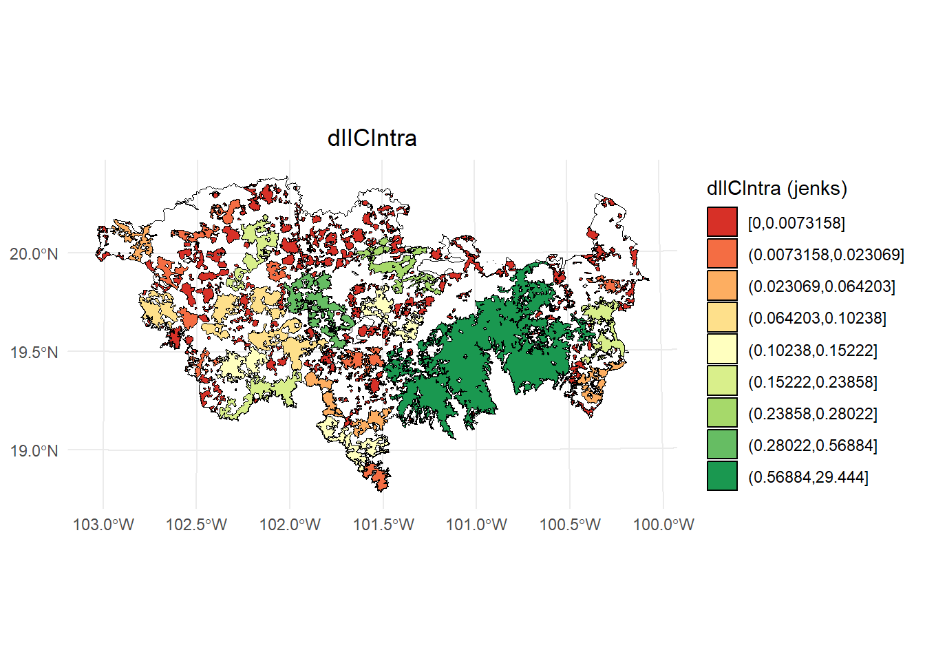
- dIICIntra
# Calcular los intervalos de Jenks para strength
breaks <- classInt::classIntervals(IIC$dIICintra, n = 9, style = "jenks")

# Crear una nueva variable categórica con los intervalos
IIC <- IIC %>%
  mutate(dIIC_q = cut(dIICintra,
                          breaks = breaks$brks,
                          include.lowest = TRUE,
                          dig.lab = 5))

# Graficar en ggplot2 usando las clases Jenks
ggplot() +
  geom_sf(data = paisaje, fill = NA, color = "black") +
  geom_sf(data = IIC, aes(fill = dIIC_q), color = "black", size = 0.1) +
  scale_fill_brewer(palette = "RdYlGn", direction = 1, name = "dIICIntra (jenks)") +
  theme_minimal() +
  labs(
    title = "dIICIntra",
    fill = "dIICIntra"
  ) +
  theme(
    legend.position = "right",
    plot.title = element_text(hjust = 0.5)
  )
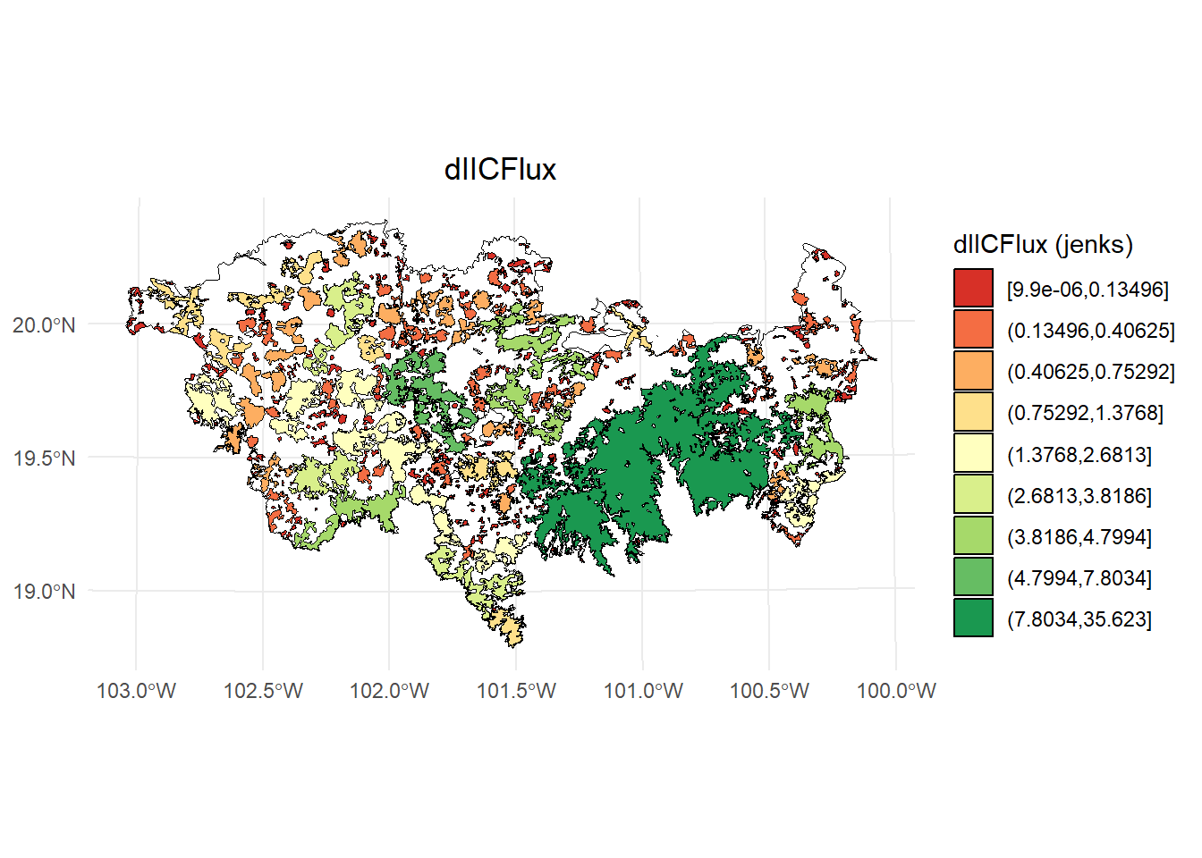
- dIICflux
# Calcular los intervalos de Jenks para strength
breaks <- classInt::classIntervals(IIC$dIICflux, n = 9, style = "jenks")

# Crear una nueva variable categórica con los intervalos
IIC <- IIC %>%
  mutate(dIIC_q = cut(dIICflux,
                          breaks = breaks$brks,
                          include.lowest = TRUE,
                          dig.lab = 5))

# Graficar en ggplot2 usando las clases Jenks
ggplot() +
  geom_sf(data = paisaje, fill = NA, color = "black") +
  geom_sf(data = IIC, aes(fill = dIIC_q), color = "black", size = 0.1) +
  scale_fill_brewer(palette = "RdYlGn", direction = 1, name = "dIICFlux (jenks)") +
  theme_minimal() +
  labs(
    title = "dIICFlux",
    fill = "dIICFlux"
  ) +
  theme(
    legend.position = "right",
    plot.title = element_text(hjust = 0.5)
  )
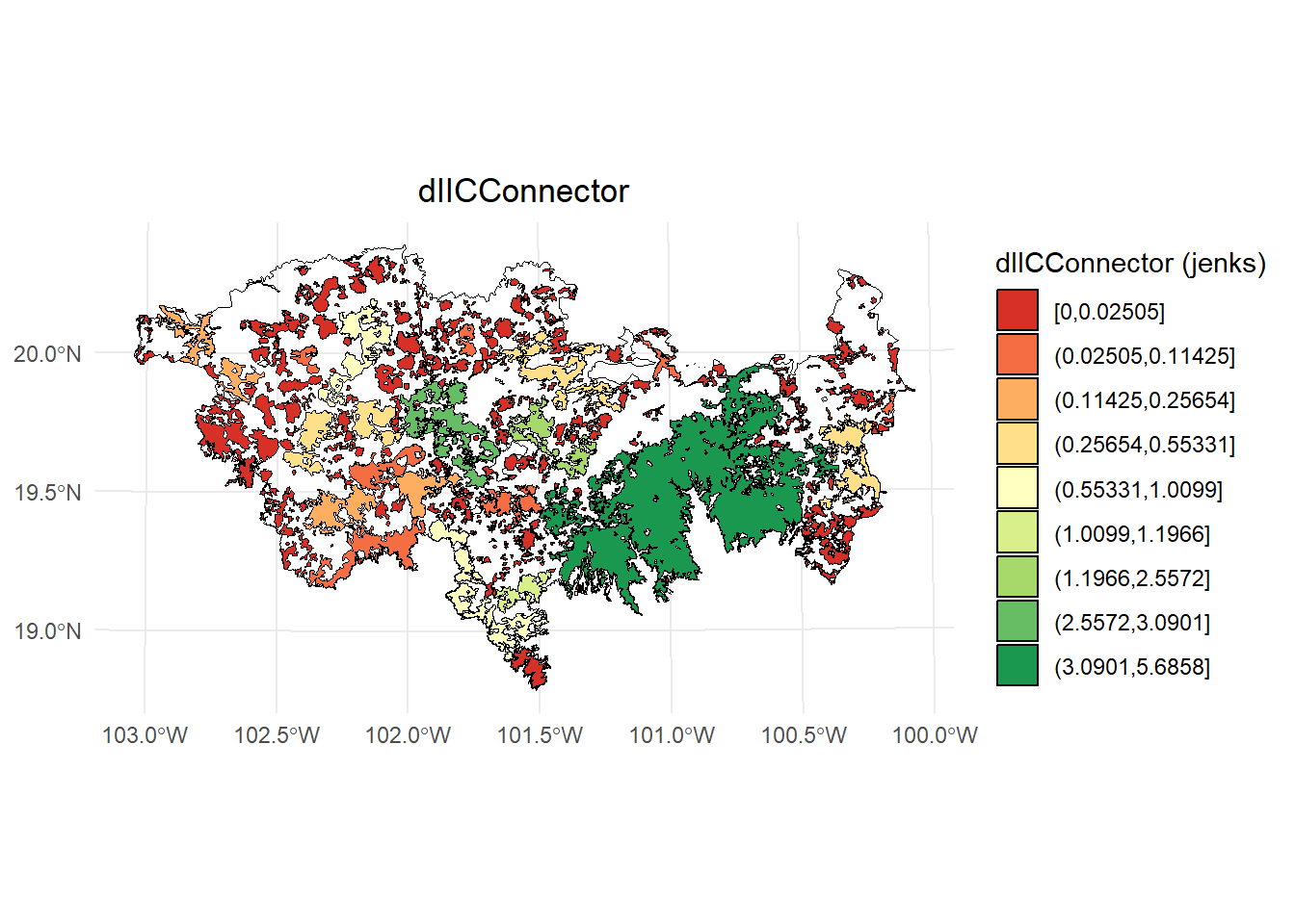
- dIICconnector
# Calcular los intervalos de Jenks para strength
breaks <- classInt::classIntervals(IIC$dIICconnector, n = 9, style = "jenks")

# Crear una nueva variable categórica con los intervalos
IIC <- IIC %>%
  mutate(dIIC_q = cut(dIICconnector,
                          breaks = breaks$brks,
                          include.lowest = TRUE,
                          dig.lab = 5))

# Graficar en ggplot2 usando las clases Jenks
ggplot() +
  geom_sf(data = paisaje, fill = NA, color = "black") +
  geom_sf(data = IIC, aes(fill = dIIC_q), color = "black", size = 0.1) +
  scale_fill_brewer(palette = "RdYlGn", direction = 1, name = "dIICConnector (jenks)") +
  theme_minimal() +
  labs(
    title = "dIICConnector",
    fill = "dIICConnector"
  ) +
  theme(
    legend.position = "right",
    plot.title = element_text(hjust = 0.5)
  )
5.8 Ejemplo 5. Distancia euclidiana: fracciones y overall
- sin usar attribute
- 10 km de mediana de dispersión
- Unidad de área en ha
area_paisaje <- st_area(paisaje)
area_paisaje <- unit_convert(area_paisaje, "m2", "ha")

IIC <- MK_dPCIIC(nodes = habitat_nodes,
                attribute = NULL,
                area_unit = "ha",
                distance = list(type = "edge", keep = 0.1),
                LA = area_paisaje,
                overall = TRUE,
                onlyoverall = FALSE,
                metric = "IIC",
                distance_thresholds = 10000,
                intern = TRUE) #10 km
#> Estimating IIC index. This may take several minutes depending on the number of nodes
#>
  |
  |                                                  |   0%
#>  ■■■■■■■■■■■■■■■■■■■■■■■■■■■       85% |  ETA:  1s
#>
#> Done!
IIC
#> $node_importances_d10000
#> Simple feature collection with 404 features and 5 fields
#> Geometry type: POLYGON
#> Dimension:     XY
#> Bounding box:  xmin: -108954 ymin: 2025032 xmax: 202330.2 ymax: 2198936
#> Projected CRS: NAD_1927_Albers
#> First 10 features:
#>    Id      dIIC dIICintra  dIICflux dIICconnector
#> 1   1 0.0067065 0.0000013 0.0067052   0.000000000
#> 2   2 0.0210320 0.0000085 0.0210235   0.000000000
#> 3   3 1.0591462 0.0213281 1.0312790   0.006539041
#> 4   4 0.0115557 0.0000026 0.0115531   0.000000000
#> 5   5 0.0254291 0.0000060 0.0254231   0.000000000
#> 6   6 0.0036214 0.0000001 0.0036212   0.000000000
#> 7   7 0.0059875 0.0000003 0.0059872   0.000000000
#> 8   8 0.0079222 0.0000006 0.0079216   0.000000000
#> 9   9 0.0280103 0.0000073 0.0280030   0.000000000
#> 10 10 4.5575494 0.1522233 3.3954709   1.009855242
#>                          geometry
#> 1  POLYGON ((54911.05 2035815,...
#> 2  POLYGON ((44591.28 2042209,...
#> 3  POLYGON ((46491.11 2042467,...
#> 4  POLYGON ((54944.49 2048163,...
#> 5  POLYGON ((80094.28 2064140,...
#> 6  POLYGON ((69205.24 2066394,...
#> 7  POLYGON ((68554.2 2066632, ...
#> 8  POLYGON ((69995.53 2066880,...
#> 9  POLYGON ((79368.68 2067324,...
#> 10 POLYGON ((23378.32 2067554,...
#>
#> $overall_d10000
#>     Index        Value
#> 1  IICnum 5.693868e+11
#> 2 EC(IIC) 7.545772e+05
#> 3     IIC 7.467188e-02
5.9 Ejemplo 6. Distancia euclidiana: varios umbrales de distancia
- sin usar attribute
- 2, 10 y 50 km de medianas de dispersión
- Unidad de área en ha
area_paisaje <- st_area(paisaje)
area_paisaje <- unit_convert(area_paisaje, "m2", "ha")

IIC <- MK_dPCIIC(nodes = habitat_nodes,
                attribute = NULL,
                area_unit = "ha",
                distance = list(type = "edge", keep = 0.1),
                LA = area_paisaje,
                overall = TRUE,
                onlyoverall = FALSE,
                metric = "IIC",
                distance_thresholds = c(2000, 10000, 50000),
                intern = TRUE)
#> Estimating IIC index. This may take several minutes depending on the number of nodes
#>
  |
  |                                                  |   0%
  |
  |                                                  |   0%
#>  ■■■■■■■■■■■■■                     38% |  ETA:  2s
#>
  |
  |=================                                 |  33%
  |
  |                                                  |   0%
#>  ■■■■■■■■■■■■■■■■■■■■■■■■■■■       87% |  ETA:  1s
#>
  |
  |=================================                 |  67%
  |
  |                                                  |   0%
#>  ■■■■■■■                           20% |  ETA:  8s
#>  ■■■■■■■■■■■■■■■■■                 54% |  ETA:  4s
#>  ■■■■■■■■■■■■■■■■■■■■■■■■■■■■      91% |  ETA:  1s
#>
  |
  |==================================================| 100%
#>
#> Done!
IIC
#> $d2000
#> $d2000$node_importances_d2000
#> Simple feature collection with 404 features and 5 fields
#> Geometry type: POLYGON
#> Dimension:     XY
#> Bounding box:  xmin: -108954 ymin: 2025032 xmax: 202330.2 ymax: 2198936
#> Projected CRS: NAD_1927_Albers
#> First 10 features:
#>    Id     dIIC dIICintra  dIICflux dIICconnector
#> 1   1 17.28636 0.0000013 0.0068969      17.27946
#> 2   2 17.29811 0.0000089 0.0204943      17.27760
#> 3   3 18.16002 0.0221965 1.0038668      17.13396
#> 4   4 17.29016 0.0000027 0.0111808      17.27897
#> 5   5 17.29788 0.0000062 0.0197837      17.27809
#> 6   6 17.28310 0.0000001 0.0028178      17.28028
#> 7   7 17.28470 0.0000003 0.0046587      17.28004
#> 8   8 17.28793 0.0000006 0.0080829      17.27985
#> 9   9 17.32364 0.0000076 0.0285784      17.29506
#> 10 10 20.91990 0.1584212 3.0660332      17.69544
#>                          geometry
#> 1  POLYGON ((54911.05 2035815,...
#> 2  POLYGON ((44591.28 2042209,...
#> 3  POLYGON ((46491.11 2042467,...
#> 4  POLYGON ((54944.49 2048163,...
#> 5  POLYGON ((80094.28 2064140,...
#> 6  POLYGON ((69205.24 2066394,...
#> 7  POLYGON ((68554.2 2066632, ...
#> 8  POLYGON ((69995.53 2066880,...
#> 9  POLYGON ((79368.68 2067324,...
#> 10 POLYGON ((23378.32 2067554,...
#>
#> $d2000$overall_d2000
#>     Index        Value
#> 1  IICnum 5.471106e+11
#> 2 EC(IIC) 7.396693e+05
#> 3     IIC 7.175048e-02
#>
#>
#> $d10000
#> $d10000$node_importances_d10000
#> Simple feature collection with 404 features and 5 fields
#> Geometry type: POLYGON
#> Dimension:     XY
#> Bounding box:  xmin: -108954 ymin: 2025032 xmax: 202330.2 ymax: 2198936
#> Projected CRS: NAD_1927_Albers
#> First 10 features:
#>    Id      dIIC dIICintra  dIICflux dIICconnector
#> 1   1 0.0067065 0.0000013 0.0067052   0.000000000
#> 2   2 0.0210320 0.0000085 0.0210235   0.000000000
#> 3   3 1.0591462 0.0213281 1.0312790   0.006539041
#> 4   4 0.0115557 0.0000026 0.0115531   0.000000000
#> 5   5 0.0254291 0.0000060 0.0254231   0.000000000
#> 6   6 0.0036214 0.0000001 0.0036212   0.000000000
#> 7   7 0.0059875 0.0000003 0.0059872   0.000000000
#> 8   8 0.0079222 0.0000006 0.0079216   0.000000000
#> 9   9 0.0280103 0.0000073 0.0280030   0.000000000
#> 10 10 4.5575494 0.1522233 3.3954709   1.009855242
#>                          geometry
#> 1  POLYGON ((54911.05 2035815,...
#> 2  POLYGON ((44591.28 2042209,...
#> 3  POLYGON ((46491.11 2042467,...
#> 4  POLYGON ((54944.49 2048163,...
#> 5  POLYGON ((80094.28 2064140,...
#> 6  POLYGON ((69205.24 2066394,...
#> 7  POLYGON ((68554.2 2066632, ...
#> 8  POLYGON ((69995.53 2066880,...
#> 9  POLYGON ((79368.68 2067324,...
#> 10 POLYGON ((23378.32 2067554,...
#>
#> $d10000$overall_d10000
#>     Index        Value
#> 1  IICnum 5.693868e+11
#> 2 EC(IIC) 7.545772e+05
#> 3     IIC 7.467188e-02
#>
#>
#> $d50000
#> $d50000$node_importances_d50000
#> Simple feature collection with 404 features and 5 fields
#> Geometry type: POLYGON
#> Dimension:     XY
#> Bounding box:  xmin: -108954 ymin: 2025032 xmax: 202330.2 ymax: 2198936
#> Projected CRS: NAD_1927_Albers
#> First 10 features:
#>    Id      dIIC dIICintra  dIICflux dIICconnector
#> 1   1 0.0108854 0.0000010 0.0108844  5.535500e-15
#> 2   2 0.0280741 0.0000064 0.0280677  4.312520e-15
#> 3   3 1.4048675 0.0159201 1.3889474  6.883380e-15
#> 4   4 0.0154866 0.0000019 0.0154847  0.000000e+00
#> 5   5 0.0241239 0.0000045 0.0241194  0.000000e+00
#> 6   6 0.0034401 0.0000001 0.0034400  9.836320e-15
#> 7   7 0.0056974 0.0000002 0.0056972  5.062790e-15
#> 8   8 0.0075250 0.0000004 0.0075246  1.169117e-14
#> 9   9 0.0265849 0.0000054 0.0265795  1.066508e-14
#> 10 10 4.1637595 0.1136249 4.0497996  3.349366e-04
#>                          geometry
#> 1  POLYGON ((54911.05 2035815,...
#> 2  POLYGON ((44591.28 2042209,...
#> 3  POLYGON ((46491.11 2042467,...
#> 4  POLYGON ((54944.49 2048163,...
#> 5  POLYGON ((80094.28 2064140,...
#> 6  POLYGON ((69205.24 2066394,...
#> 7  POLYGON ((68554.2 2066632, ...
#> 8  POLYGON ((69995.53 2066880,...
#> 9  POLYGON ((79368.68 2067324,...
#> 10 POLYGON ((23378.32 2067554,...
#>
#> $d50000$overall_d50000
#>     Index        Value
#> 1  IICnum 7.628072e+11
#> 2 EC(IIC) 8.733883e+05
#> 3 IIC 1.000379e-015.11 Ejemplo 1. Distancia euclidiana
- Sin usar LA
- sin usar attribute
- 10 km de mediana de dispersión con una probabilidad de 0.5
- Unidad de área en ha
- Solo índice para todo el paisaje
PC <- MK_dPCIIC(nodes = habitat_nodes,
                attribute = NULL,
                area_unit = "ha",
                distance = list(type = "edge", keep = 0.1),
                LA = NULL,
                onlyoverall = TRUE,
                metric = "PC",
                probability = 0.5,
                distance_thresholds = 10000,
                intern = TRUE) #10 km
#> Estimating PC index. This may take several minutes depending on the number of nodes
#>
  |
  |                                                  |   0%
  |
  |==================================================| 100%
#>
#> Done!
PC
#>    Index        Value
#> 1  PCnum 1.301622e+12
#> 2 EC(PC) 1.140887e+06
5.12 Ejemplo 2. Distancia euclidiana
- sin usar attribute
- 10 km de mediana de dispersión con una probabilidad de 0.5
- Unidad de área en ha
- Solo índice para todo el paisaje
area_paisaje <- st_area(paisaje)
area_paisaje <- unit_convert(area_paisaje, "m2", "ha")

PC <- MK_dPCIIC(nodes = habitat_nodes,
                attribute = NULL,
                area_unit = "ha",
                distance = list(type = "centroid"),
                LA = area_paisaje,
                onlyoverall = TRUE,
                metric = "PC",
                probability = 0.5,
                distance_thresholds = 10000,
                intern = TRUE) #10 km
#> Estimating PC index. This may take several minutes depending on the number of nodes
#>
  |
  |                                                  |   0%
  |
  |==================================================| 100%
#>
#> Done!
PC
#>    Index        Value
#> 1  PCnum 2.136028e+11
#> 2 EC(PC) 4.621718e+05
#> 3     PC 2.801281e-02
5.13 Ejemplo 3. Distancia euclidiana: fracciones
- sin usar attribute
- 10 km de mediana de dispersión con una probabilidad de 0.5
- Unidad de área en ha
area_paisaje <- st_area(paisaje)
area_paisaje <- unit_convert(area_paisaje, "m2", "ha")

PC <- MK_dPCIIC(nodes = habitat_nodes,
                attribute = NULL,
                area_unit = "ha",
                distance = list(type = "edge", keep = 0.1),
                LA = area_paisaje,
                onlyoverall = FALSE,
                metric = "PC",
                probability = 0.5,
                distance_thresholds = 10000,
                intern = TRUE) #10 km
#> Estimating PC index. This may take several minutes depending on the number of nodes
#>
  |
  |                                                  |   0%
  |
  |==================================================| 100%
#>  ■■■■                               9% |  ETA: 37s
#>  ■■■■■■                            16% |  ETA: 34s
#>  ■■■■■■■■                          22% |  ETA: 34s
#>  ■■■■■■■■■                         26% |  ETA: 35s
#>  ■■■■■■■■■■                        31% |  ETA: 34s
#>  ■■■■■■■■■■■■                      37% |  ETA: 32s
#>  ■■■■■■■■■■■■■■                    43% |  ETA: 29s
#>  ■■■■■■■■■■■■■■■                   48% |  ETA: 27s
#>  ■■■■■■■■■■■■■■■■■                 54% |  ETA: 24s
#>  ■■■■■■■■■■■■■■■■■■■               60% |  ETA: 21s
#>  ■■■■■■■■■■■■■■■■■■■■■             66% |  ETA: 17s
#>  ■■■■■■■■■■■■■■■■■■■■■■■           73% |  ETA: 14s
#>  ■■■■■■■■■■■■■■■■■■■■■■■■■         79% |  ETA: 11s
#>  ■■■■■■■■■■■■■■■■■■■■■■■■■■        85% |  ETA:  8s
#>  ■■■■■■■■■■■■■■■■■■■■■■■■■■■■      91% |  ETA:  5s
#>  ■■■■■■■■■■■■■■■■■■■■■■■■■■■■■■    96% |  ETA:  2s
#>
#> Done!
PC
#> Simple feature collection with 404 features and 5 fields
#> Geometry type: POLYGON
#> Dimension:     XY
#> Bounding box:  xmin: -108954 ymin: 2025032 xmax: 202330.2 ymax: 2198936
#> Projected CRS: NAD_1927_Albers
#> First 10 features:
#>    Id       dPC  dPCintra   dPCflux dPCconnector
#> 1   1 0.0128564 0.0000006 0.0128558 0.000000e+00
#> 2   2 0.0332059 0.0000037 0.0332022 0.000000e+00
#> 3   3 1.6831849 0.0093299 1.6665804 7.274621e-03
#> 4   4 0.0184037 0.0000011 0.0184026 0.000000e+00
#> 5   5 0.0285162 0.0000026 0.0285136 0.000000e+00
#> 6   6 0.0040938 0.0000001 0.0040937 5.309968e-08
#> 7   7 0.0069481 0.0000001 0.0068704 7.758334e-05
#> 8   8 0.0088543 0.0000003 0.0088540 0.000000e+00
#> 9   9 0.0369150 0.0000032 0.0331109 3.800919e-03
#> 10 10 5.5556530 0.0665892 4.4246468 1.064417e+00
#>                          geometry
#> 1  POLYGON ((54911.05 2035815,...
#> 2  POLYGON ((44591.28 2042209,...
#> 3  POLYGON ((46491.11 2042467,...
#> 4  POLYGON ((54944.49 2048163,...
#> 5  POLYGON ((80094.28 2064140,...
#> 6  POLYGON ((69205.24 2066394,...
#> 7  POLYGON ((68554.2 2066632, ...
#> 8  POLYGON ((69995.53 2066880,...
#> 9  POLYGON ((79368.68 2067324,...
#> 10 POLYGON ((23378.32 2067554,...
Exploremos un plot usando intervalos:
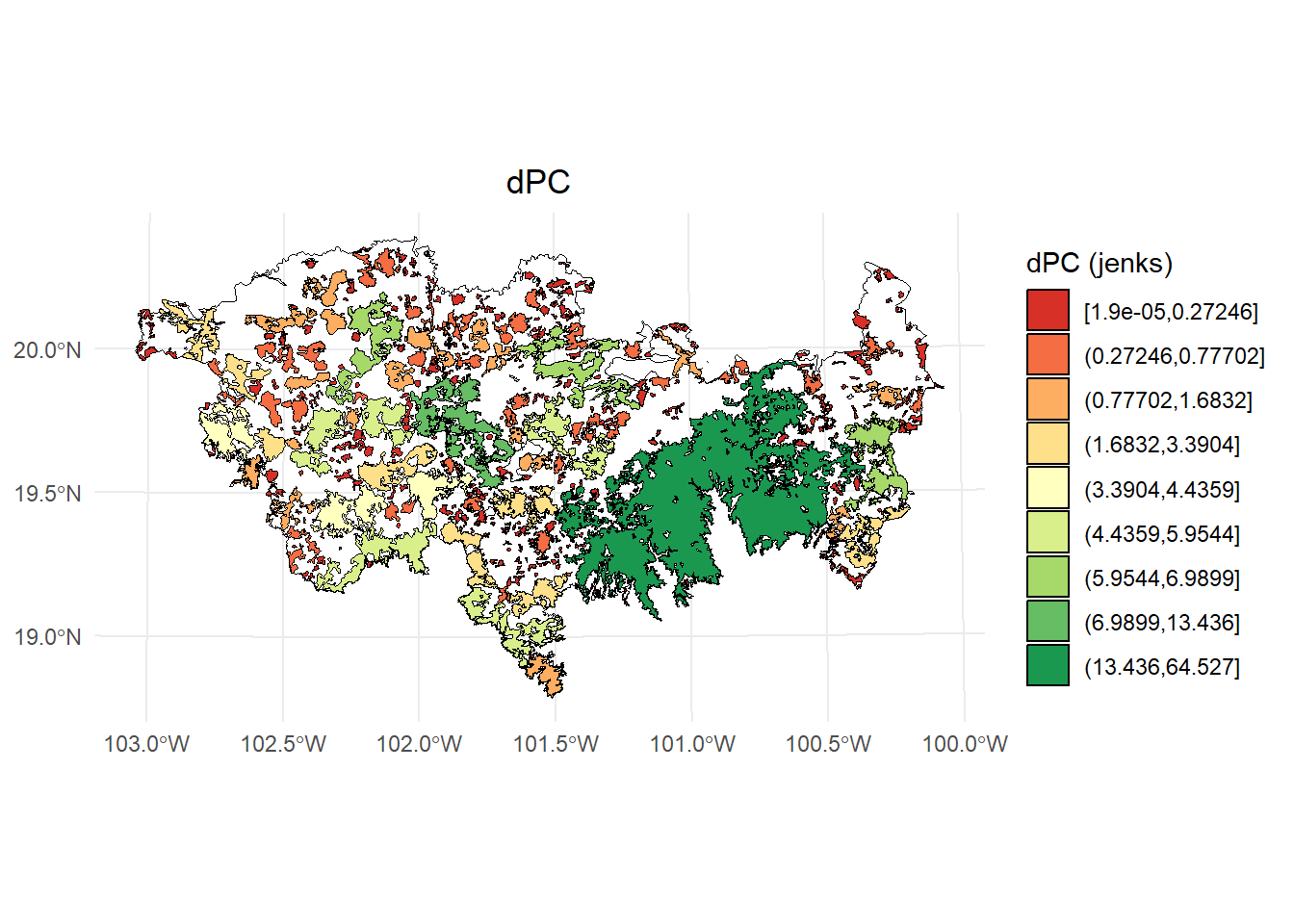
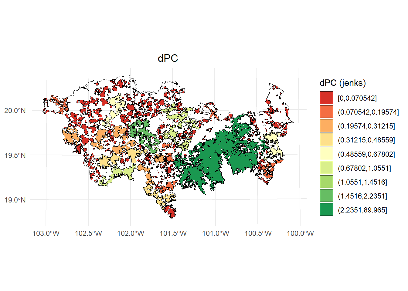
- dPC
library(classInt)
library(dplyr)

# Calcular los intervalos de Jenks para strength
breaks <- classInt::classIntervals(PC$dPC, n = 9, style = "jenks")

# Crear una nueva variable categórica con los intervalos
PC <- PC %>%
  mutate(dPC_q = cut(dPC,
                          breaks = breaks$brks,
                          include.lowest = TRUE,
                          dig.lab = 5))

# Graficar en ggplot2 usando las clases Jenks
ggplot() +
  geom_sf(data = paisaje, fill = NA, color = "black") +
  geom_sf(data = PC, aes(fill = dPC_q), color = "black", size = 0.1) +
  scale_fill_brewer(palette = "RdYlGn", direction = 1, name = "dPC (jenks)") +
  theme_minimal() +
  labs(
    title = "dPC",
    fill = "dPC"
  ) +
  theme(
    legend.position = "right",
    plot.title = element_text(hjust = 0.5)
  )
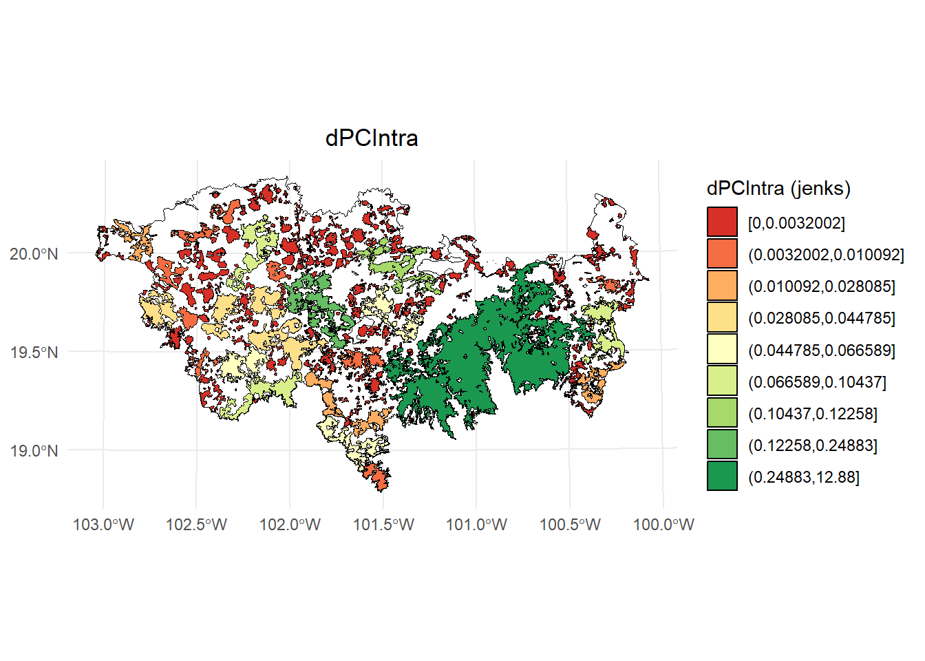
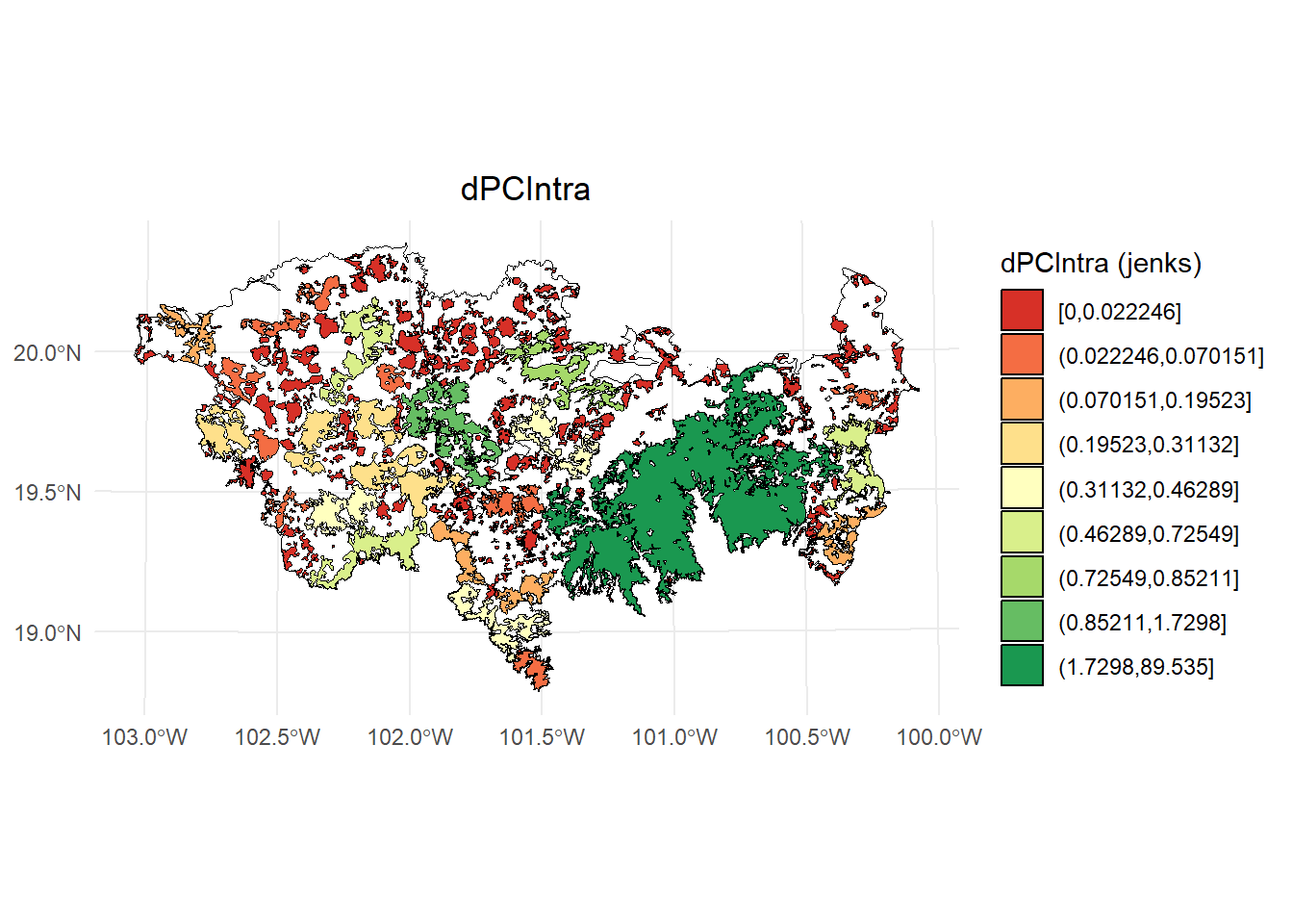
- dPCIntra
# Calcular los intervalos de Jenks para strength
breaks <- classInt::classIntervals(PC$dPCintra, n = 9, style = "jenks")

# Crear una nueva variable categórica con los intervalos
PC <- PC %>%
  mutate(dPC_q = cut(dPCintra,
                      breaks = breaks$brks,
                      include.lowest = TRUE,
                      dig.lab = 5))

# Graficar en ggplot2 usando las clases Jenks
ggplot() +
  geom_sf(data = paisaje, fill = NA, color = "black") +
  geom_sf(data = PC, aes(fill = dPC_q), color = "black", size = 0.1) +
  scale_fill_brewer(palette = "RdYlGn", direction = 1, name = "dPCIntra (jenks)") +
  theme_minimal() +
  labs(
    title = "dPCIntra",
    fill = "dPCIntra"
  ) +
  theme(
    legend.position = "right",
    plot.title = element_text(hjust = 0.5)
  )
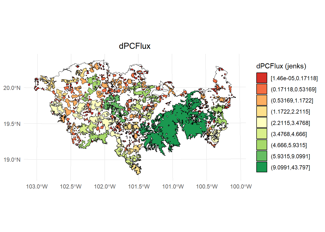
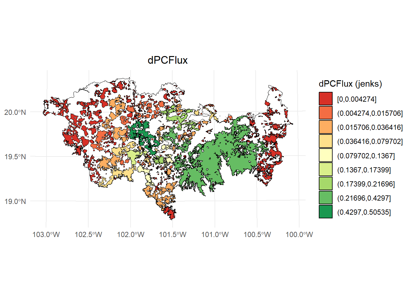
- dPCflux
# Calcular los intervalos de Jenks para strength
breaks <- classInt::classIntervals(PC$dPCflux, n = 9, style = "jenks")

# Crear una nueva variable categórica con los intervalos
PC <- PC %>%
  mutate(dPC_q = cut(dPCflux,
                      breaks = breaks$brks,
                      include.lowest = TRUE,
                      dig.lab = 5))

# Graficar en ggplot2 usando las clases Jenks
ggplot() +
  geom_sf(data = paisaje, fill = NA, color = "black") +
  geom_sf(data = PC, aes(fill = dPC_q), color = "black", size = 0.1) +
  scale_fill_brewer(palette = "RdYlGn", direction = 1, name = "dPCFlux (jenks)") +
  theme_minimal() +
  labs(
    title = "dPCFlux",
    fill = "dPCFlux"
  ) +
  theme(
    legend.position = "right",
    plot.title = element_text(hjust = 0.5)
  )
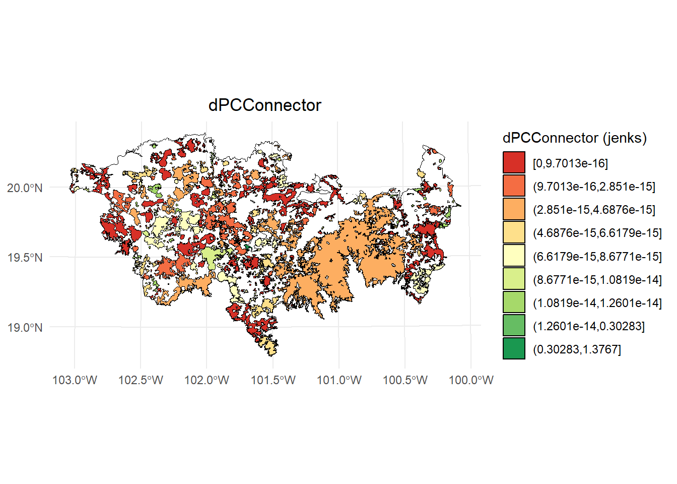
- dPCconnector
# Calcular los intervalos de Jenks para strength
breaks <- classInt::classIntervals(PC$dPCconnector, n = 9, style = "jenks")

# Crear una nueva variable categórica con los intervalos
PC <- PC %>%
  mutate(dPC_q = cut(dPCconnector,
                     breaks = breaks$brks,
                     include.lowest = TRUE,
                     dig.lab = 5))

# Graficar en ggplot2 usando las clases Jenks
ggplot() +
  geom_sf(data = paisaje, fill = NA, color = "black") +
  geom_sf(data = PC, aes(fill = dPC_q), color = "black", size = 0.1) +
  scale_fill_brewer(palette = "RdYlGn", direction = 1, name = "dPCConnector (jenks)") +
  theme_minimal() +
  labs(
    title = "dPCConnector",
    fill = "dPCConnector"
  ) +
  theme(
    legend.position = "right",
    plot.title = element_text(hjust = 0.5)
  )
5.14 Ejemplo 4. Distancia euclidiana: fracciones y overall
- sin usar attribute
- 10 km de mediana de dispersión con una probabilidad de 0.5
- Unidad de área en ha
area_paisaje <- st_area(paisaje)
area_paisaje <- unit_convert(area_paisaje, "m2", "ha")

PC <- MK_dPCIIC(nodes = habitat_nodes,
                attribute = NULL,
                area_unit = "ha",
                distance = list(type = "edge", keep = 0.1),
                LA = area_paisaje,
                overall = TRUE,
                onlyoverall = FALSE,
                metric = "PC",
                probability = 0.5,
                distance_thresholds = 10000,
                intern = TRUE) #10 km
#> Estimating PC index. This may take several minutes depending on the number of nodes
#>
  |
  |                                                  |   0%
  |
  |==================================================| 100%
#>  ■■                                 4% |  ETA: 30s
#>  ■■■■                              11% |  ETA: 36s
#>  ■■■■■■                            18% |  ETA: 33s
#>  ■■■■■■■■■                         25% |  ETA: 30s
#>  ■■■■■■■■■■                        31% |  ETA: 29s
#>  ■■■■■■■■■■■■                      37% |  ETA: 27s
#>  ■■■■■■■■■■■■■■                    43% |  ETA: 26s
#>  ■■■■■■■■■■■■■■■                   47% |  ETA: 25s
#>  ■■■■■■■■■■■■■■■■                  51% |  ETA: 24s
#>  ■■■■■■■■■■■■■■■■■■                57% |  ETA: 21s
#>  ■■■■■■■■■■■■■■■■■■■■              64% |  ETA: 18s
#>  ■■■■■■■■■■■■■■■■■■■■■■            69% |  ETA: 16s
#>  ■■■■■■■■■■■■■■■■■■■■■■■           75% |  ETA: 12s
#>  ■■■■■■■■■■■■■■■■■■■■■■■■■■        82% |  ETA:  9s
#>  ■■■■■■■■■■■■■■■■■■■■■■■■■■■       88% |  ETA:  6s
#>  ■■■■■■■■■■■■■■■■■■■■■■■■■■■■■■    96% |  ETA:  2s
#>
#> Done!
PC
#> $node_importances_d10000
#> Simple feature collection with 404 features and 5 fields
#> Geometry type: POLYGON
#> Dimension:     XY
#> Bounding box:  xmin: -108954 ymin: 2025032 xmax: 202330.2 ymax: 2198936
#> Projected CRS: NAD_1927_Albers
#> First 10 features:
#>    Id       dPC  dPCintra   dPCflux dPCconnector
#> 1   1 0.0128564 0.0000006 0.0128558 0.000000e+00
#> 2   2 0.0332059 0.0000037 0.0332022 0.000000e+00
#> 3   3 1.6831849 0.0093299 1.6665804 7.274621e-03
#> 4   4 0.0184037 0.0000011 0.0184026 0.000000e+00
#> 5   5 0.0285162 0.0000026 0.0285136 0.000000e+00
#> 6   6 0.0040938 0.0000001 0.0040937 5.309968e-08
#> 7   7 0.0069481 0.0000001 0.0068704 7.758334e-05
#> 8   8 0.0088543 0.0000003 0.0088540 0.000000e+00
#> 9   9 0.0369150 0.0000032 0.0331109 3.800919e-03
#> 10 10 5.5556530 0.0665892 4.4246468 1.064417e+00
#>                          geometry
#> 1  POLYGON ((54911.05 2035815,...
#> 2  POLYGON ((44591.28 2042209,...
#> 3  POLYGON ((46491.11 2042467,...
#> 4  POLYGON ((54944.49 2048163,...
#> 5  POLYGON ((80094.28 2064140,...
#> 6  POLYGON ((69205.24 2066394,...
#> 7  POLYGON ((68554.2 2066632, ...
#> 8  POLYGON ((69995.53 2066880,...
#> 9  POLYGON ((79368.68 2067324,...
#> 10 POLYGON ((23378.32 2067554,...
#>
#> $overall_d10000
#>    Index        Value
#> 1  PCnum 1.301622e+12
#> 2 EC(PC) 1.140887e+06
#> 3     PC 1.707004e-01
5.15 Ejemplo 5. Distancia euclidiana: paralelizar
- sin usar attribute
- 10 km de mediana de dispersión con una probabilidad de 0.5
- Unidad de área en ha
El argumento parallel solo se activa si tienes más de 2000 parches. Si tienes menos de 4000 parches utiliza parallel_mode = 1.
PC <- MK_dPCIIC(nodes = habitat_nodes,
                attribute = NULL,
                area_unit = "ha",
                distance = list(type = "edge", keep = 0.1),
                LA = area_paisaje,
                onlyoverall = FALSE,
                metric = "PC",
                probability = 0.5,
                distance_thresholds = 10000,
                parallel = 4,
                parallel_mode = 1,
                intern = TRUE) #10 km
PC
Siempre utiliza la mitad de tus cores disponibles en tu máquina, es decir si son 12 los cores totales utiliza 6. También puedes restar uno o dos cores del total, es decir, si son 12 los totales utiliza 11 o 10.
# Conocer numero de Cores de tu maquina
library(parallel)
parallel::detectCores()
#> [1] 22
5.16 Ejemplo 6. Distancia costo
- sin usar attribute
- 10 km de mediana de dispersión con una probabilidad de 0.5
- Unidad de área en ha
- Usa un raster con valores de resistencia al movimiento
- Para este ejemplo solo estimaremos los valores a nivel de parche
La resistencia del paisaje a la dispersión se estimó con una resolución de 100 metros utilizando un índice espacial de huella humana, intensidad del uso del suelo, tiempo de intervención humana en el paisaje, vulnerabilidad biofísica, fragmentación y pérdida de hábitat (Correa Ayram et al., 2017, https://doi.org/10.1016/j.ecolind.2016.09.007). El raster se agregó usando un factor de 5 para cambiar su resolución original de 100 m a 500 m.
library(terra)
#> terra 1.8.29
#>
#> Adjuntando el paquete: 'terra'
#> The following objects are masked from 'package:igraph':
#>
#>     blocks, compare
data("resistance_matrix", package = "Makurhini")

raster_map <- as(resistance_matrix, "SpatialPixelsDataFrame")
raster_map <- as.data.frame(raster_map)
colnames(raster_map) <- c("value", "x", "y")
ggplot() +
  geom_tile(data = raster_map, aes(x = x, y = y, fill = value), alpha = 0.8) +
  geom_sf(data = paisaje, aes(color = "Study area"), fill = NA, color = "black") +
  geom_sf(data = habitat_nodes, aes(color = "Habitat nodes"), fill = "forestgreen", linewidth = 0.5) +
  scale_fill_gradientn(colors = c("#000004FF", "#1B0C42FF", "#4B0C6BFF", "#781C6DFF",
                                  "#A52C60FF", "#CF4446FF", "#ED6925FF", "#FB9A06FF",
                                  "#F7D03CFF", "#FCFFA4FF"))+
  scale_color_manual(name = "", values = "black")+
  theme_minimal() +
  theme(axis.title.x = element_blank(),
        axis.title.y = element_blank())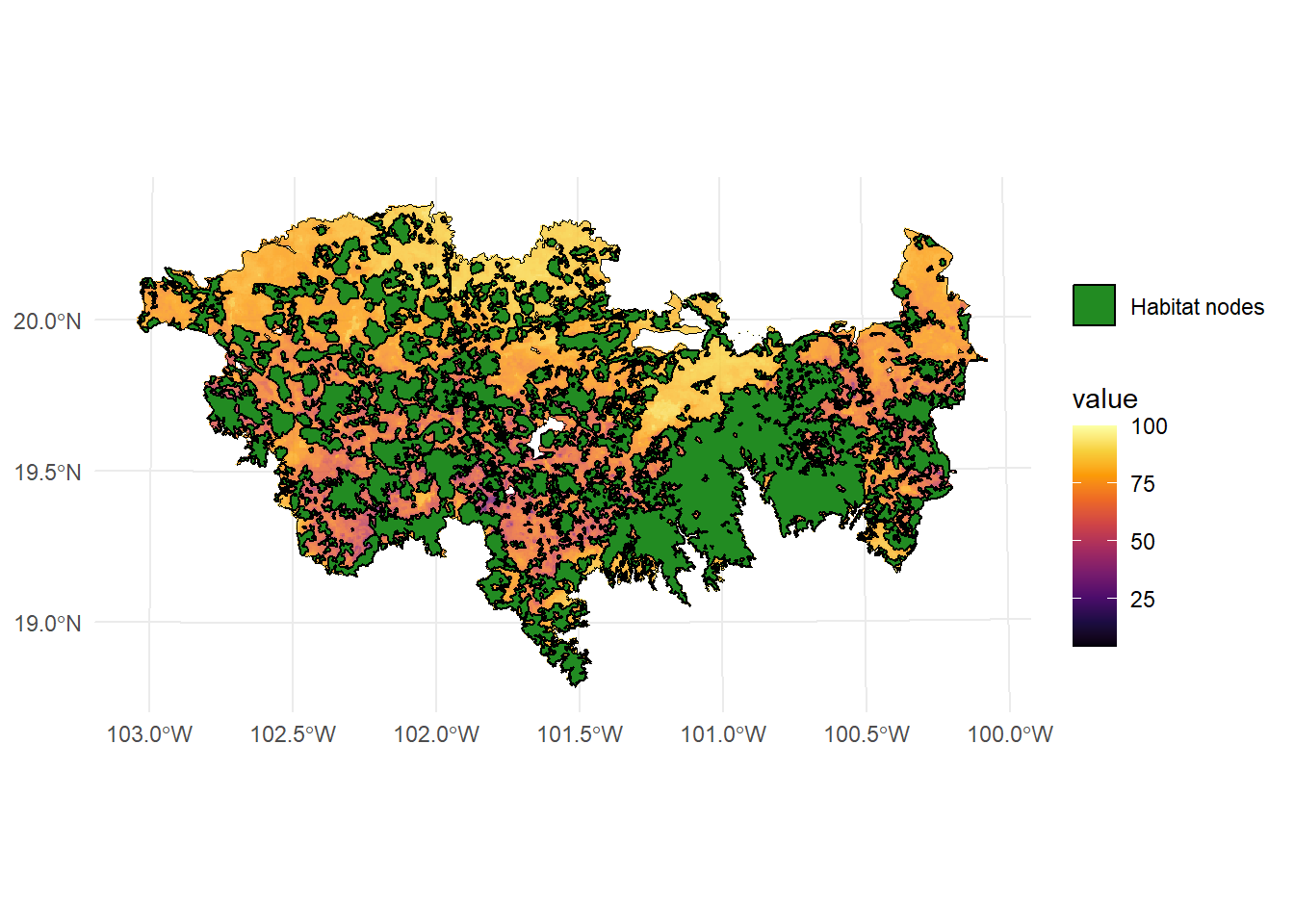
Estamos utilizando un raster de resistencia que esta incluido en el paquete Makurhini. Para cargar un raster de resistencia para tu estudio puedes utilizar la función raster() del paquete raster o la función rast() del paquete terra.
library(raster)
resistance_matrix <- raster("direccion/nombre.tif") #puedes usar otras extensiones raster

library(terra)
resistance_matrix <- rast("direccion/nombre.tif")
Se utiliza el tipo de distancia de menor costo type = "least-cost" y al usar una distancia de resistencia se tiene que usar el otro argumento resistance, es decir, resistance = resistance_matrix.
PC <- MK_dPCIIC(nodes = habitat_nodes,
                attribute = NULL,
                distance = list(type = "least-cost",
                                resistance = resistance_matrix),
                metric = "PC", probability = 0.5,
                overall = FALSE,
                distance_thresholds = 10000) # 10 km
#> Estimating distances. This may take several minutes depending on the number of nodes and raster resolution
#> Estimating PC index. This may take several minutes depending on the number of nodes
#>
  |
  |                                                  |   0%
  |
  |==================================================| 100%
#>  ■■■■                               9% |  ETA: 12s
#>  ■■■■■■■■■■                        29% |  ETA: 10s
#>  ■■■■■■■■■■■■■■■■                  49% |  ETA:  7s
#>  ■■■■■■■■■■■■■■■■■■■■■             68% |  ETA:  5s
#>  ■■■■■■■■■■■■■■■■■■■■■■■■■■        83% |  ETA:  3s
#>
#> Done!
PC
#> Simple feature collection with 404 features and 5 fields
#> Geometry type: POLYGON
#> Dimension:     XY
#> Bounding box:  xmin: -108954 ymin: 2025032 xmax: 202330.2 ymax: 2198936
#> Projected CRS: NAD_1927_Albers
#> First 10 features:
#>    Id       dPC  dPCintra   dPCflux dPCconnector
#> 1   1 0.0000236 0.0000039 0.0000196 0.000000e+00
#> 2   2 0.0001155 0.0000259 0.0000896 0.000000e+00
#> 3   3 0.0674996 0.0648562 0.0026434 4.982560e-15
#> 4   4 0.0000722 0.0000078 0.0000644 0.000000e+00
#> 5   5 0.0001142 0.0000182 0.0000959 1.173850e-15
#> 6   6 0.0000277 0.0000004 0.0000273 0.000000e+00
#> 7   7 0.0000471 0.0000010 0.0000461 1.153109e-14
#> 8   8 0.0000596 0.0000018 0.0000579 0.000000e+00
#> 9   9 0.0001505 0.0000221 0.0001284 4.687580e-15
#> 10 10 0.4855924 0.4628919 0.0227005 6.487900e-16
#>                          geometry
#> 1  POLYGON ((54911.05 2035815,...
#> 2  POLYGON ((44591.28 2042209,...
#> 3  POLYGON ((46491.11 2042467,...
#> 4  POLYGON ((54944.49 2048163,...
#> 5  POLYGON ((80094.28 2064140,...
#> 6  POLYGON ((69205.24 2066394,...
#> 7  POLYGON ((68554.2 2066632, ...
#> 8  POLYGON ((69995.53 2066880,...
#> 9  POLYGON ((79368.68 2067324,...
#> 10 POLYGON ((23378.32 2067554,...
library(classInt)
library(dplyr)

# Calcular los intervalos de Jenks para strength
breaks <- classInt::classIntervals(PC$dPC, n = 9, style = "jenks")

# Crear una nueva variable categórica con los intervalos
PC <- PC %>%
  mutate(dPC_q = cut(dPC,
                          breaks = breaks$brks,
                          include.lowest = TRUE,
                          dig.lab = 5))

# Graficar en ggplot2 usando las clases Jenks
ggplot() +
  geom_sf(data = paisaje, fill = NA, color = "black") +
  geom_sf(data = PC, aes(fill = dPC_q), color = "black", size = 0.1) +
  scale_fill_brewer(palette = "RdYlGn", direction = 1, name = "dPC (jenks)") +
  theme_minimal() +
  labs(
    title = "dPC",
    fill = "dPC"
  ) +
  theme(
    legend.position = "right",
    plot.title = element_text(hjust = 0.5)
  )
- dPCIntra
# Calcular los intervalos de Jenks para strength
breaks <- classInt::classIntervals(PC$dPCintra, n = 9, style = "jenks")

# Crear una nueva variable categórica con los intervalos
PC <- PC %>%
  mutate(dPC_q = cut(dPCintra,
                      breaks = breaks$brks,
                      include.lowest = TRUE,
                      dig.lab = 5))

# Graficar en ggplot2 usando las clases Jenks
ggplot() +
  geom_sf(data = paisaje, fill = NA, color = "black") +
  geom_sf(data = PC, aes(fill = dPC_q), color = "black", size = 0.1) +
  scale_fill_brewer(palette = "RdYlGn", direction = 1, name = "dPCIntra (jenks)") +
  theme_minimal() +
  labs(
    title = "dPCIntra",
    fill = "dPCIntra"
  ) +
  theme(
    legend.position = "right",
    plot.title = element_text(hjust = 0.5)
  )
- dPCflux
# Calcular los intervalos de Jenks para strength
breaks <- classInt::classIntervals(PC$dPCflux, n = 9, style = "jenks")

# Crear una nueva variable categórica con los intervalos
PC <- PC %>%
  mutate(dPC_q = cut(dPCflux,
                      breaks = breaks$brks,
                      include.lowest = TRUE,
                      dig.lab = 5))

# Graficar en ggplot2 usando las clases Jenks
ggplot() +
  geom_sf(data = paisaje, fill = NA, color = "black") +
  geom_sf(data = PC, aes(fill = dPC_q), color = "black", size = 0.1) +
  scale_fill_brewer(palette = "RdYlGn", direction = 1, name = "dPCFlux (jenks)") +
  theme_minimal() +
  labs(
    title = "dPCFlux",
    fill = "dPCFlux"
  ) +
  theme(
    legend.position = "right",
    plot.title = element_text(hjust = 0.5)
  )
- dPCconnector
# Calcular los intervalos de Jenks para strength
breaks <- classInt::classIntervals(PC$dPCconnector, n = 9, style = "jenks")

# Crear una nueva variable categórica con los intervalos
PC <- PC %>%
  mutate(dPC_q = cut(dPCconnector,
                     breaks = breaks$brks,
                     include.lowest = TRUE,
                     dig.lab = 5))

# Graficar en ggplot2 usando las clases Jenks
ggplot() +
  geom_sf(data = paisaje, fill = NA, color = "black") +
  geom_sf(data = PC, aes(fill = dPC_q), color = "black", size = 0.1) +
  scale_fill_brewer(palette = "RdYlGn", direction = 1, name = "dPCConnector (jenks)") +
  theme_minimal() +
  labs(
    title = "dPCConnector",
    fill = "dPCConnector"
  ) +
  theme(
    legend.position = "right",
    plot.title = element_text(hjust = 0.5)
  )
5.17 Ejemplo 7. Distancia costo en Java
Se utiliza el tipo de distancia de menor costo type = "least-cost" y al usar una distancia de resistencia se tiene que usar el otro argumento resistance. Sin embargo, la resistencia tiene que tener solo valores enteros y no decimales. Se debe utilizar el argumento least_cost.java = TRUE. Además puedes usar cores.java = numero de cores para paralelizar el proceso y ram.java = memoria ram para estimar las distancias.
#Convertimos la resistencia a valores enteros
resist2 <- resistance_matrix
resist2 <- round(resistance_matrix)


PC <- MK_dPCIIC(nodes = habitat_nodes,
                attribute = NULL,
                distance = list(type = "least-cost",
                                resistance = resist2,
                                least_cost.java = TRUE,
                                cores.java = 2,
                                ram.java = NULL),
                metric = "PC", probability = 0.5,
                overall = TRUE,
                distance_thresholds = 40000) # 40 km
PC
5.18 Ejemplo 8. Usando nodos en formato raster
Estamos utilizando un raster de nodos que esta incluido en el paquete Makurhini. Para cargar un raster de nodos para tu estudio puedes utilizar la función raster() del paquete raster o la función rast() del paquete terra.
library(raster)
habitat_nodes_raster <- raster("direccion/nombre.tif") #puedes usar otras extensiones raster

library(terra)
habitat_nodes_raster <- rast("direccion/nombre.tif")
PC <- MK_dPCIIC(nodes = habitat_nodes_raster,
attribute = NULL,
distance = list(type = "centroid"),
metric = "PC", probability = 0.5,
overall = TRUE,
distance_thresholds = 40000) # 40 km
#> Estimating PC index. This may take several minutes depending on the number of nodes
#>
|
| | 0%
|
|==================================================| 100%
#> ■■■■■■■■ 23% | ETA: 9s
#> ■■■■■■■■■■■■■■ 45% | ETA: 7s
#> ■■■■■■■■■■■■■■■■■■■■■ 66% | ETA: 5s
#> ■■■■■■■■■■■■■■■■■■■■■■■■■■ 85% | ETA: 2s
#>
#> Done!
PC$overall_d40000
#> Index Value
#> 1 PCnum 5.116326e+19
#> 2 EC(PC) 7.152850e+09
PC$node_importances_d40000
#> class : RasterStack
#> dimensions : 357, 624, 222768, 5 (nrow, ncol, ncell, nlayers)
#> resolution : 500, 500 (x, y)
#> extent : -109586.4, 202413.6, 2024737, 2203237 (xmin, xmax, ymin, ymax)
#> crs : +proj=aea +lat_0=0 +lon_0=-102 +lat_1=17.5 +lat_2=29.5 +x_0=0 +y_0=0 +datum=NAD27 +units=m +no_defs
#> names : Id, dPC, dPCintra, dPCflux, dPCconnector
#> min values : 1.0000000, 0.0020195, 0.0000001, 0.0020194, 0.0000000
#> max values : 4.040000e+02, 5.778878e+01, 3.274351e+01, 2.504527e+01, 9.513220e-15
plot(PC$node_importances_d40000)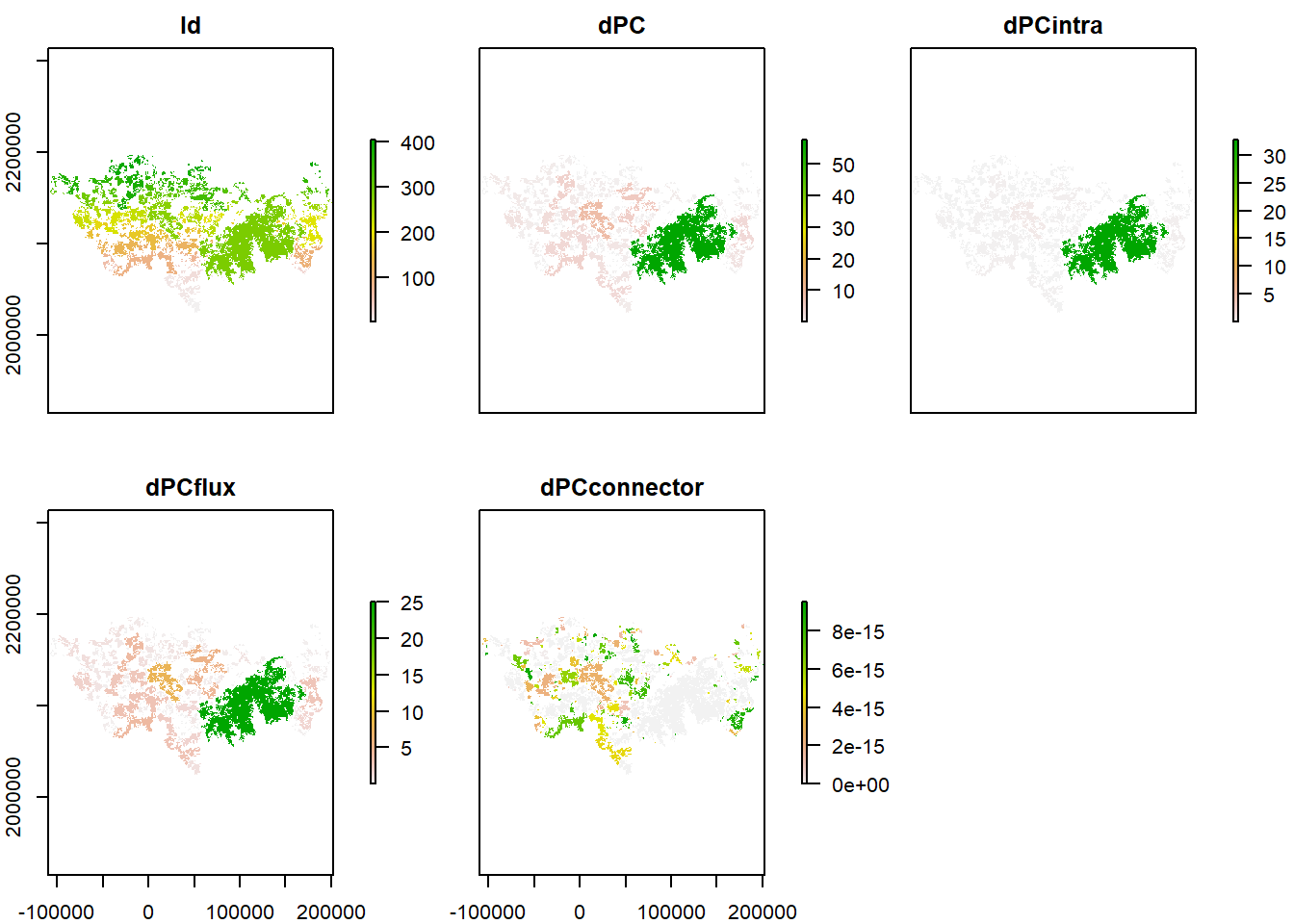
5.19 Guardar IIC o PC
Para guardar puedes usar el argumento write que necesita la ruta de la carpeta y un prefijo sin la extensión, e.g., C:/Carpeta/nombreprefijo
IIC <- MK_dPCIIC(nodes = habitat_nodes,
                 attribute = NULL,
                 area_unit = "ha",
                 distance = list(type = "edge", keep = 0.1),
                 LA = area_paisaje,
                 overall = FALSE,
                 onlyoverall = FALSE,
                 metric = "IIC",
                 distance_thresholds = 10000,
                 write = "C:/Users/tapir",
                 intern = TRUE) #10 km}
Todos los resultados se guardaran en la carpeta Users y tendran el nombre tapir
Otra forma de exportar los resultados es hacer uso de la función write_sf() del paquete sf
IIC <- MK_dPCIIC(nodes = habitat_nodes,
                 attribute = NULL,
                 area_unit = "ha",
                 distance = list(type = "edge", keep = 0.1),
                 LA = area_paisaje,
                 overall = FALSE,
                 onlyoverall = FALSE,
                 metric = "IIC",
                 distance_thresholds = 10000,
                 intern = TRUE) #10 km}

write_sf(IIC, "C:/Users/tapir.shp")
Si estimas además el overall puedes usar la función write.csv() para exportar la tabla
IIC <- MK_dPCIIC(nodes = habitat_nodes,
                 attribute = NULL,
                 area_unit = "ha",
                 distance = list(type = "edge", keep = 0.1),
                 LA = area_paisaje,
                 overall = TRUE,
                 onlyoverall = FALSE,
                 metric = "IIC",
                 distance_thresholds = 10000,
                 intern = TRUE) #10 km}

write_sf(IIC$node_importances_d10000, "C:/Users/tapir.shp")

write.csv(IIC$overall_d10000, "C:/Users/tapir.csv")
Si estimas el índice con más de un umbral de distancia
IIC <- MK_dPCIIC(nodes = habitat_nodes,
                 attribute = NULL,
                 area_unit = "ha",
                 distance = list(type = "edge", keep = 0.1),
                 LA = area_paisaje,
                 overall = TRUE,
                 onlyoverall = FALSE,
                 metric = "IIC",
                 distance_thresholds = c(10000, 20000),
                 intern = TRUE) #10 km}

write_sf(IIC$d10000$node_importances_d10000, "C:/Users/tapir10.shp")
write_sf(IIC$d20000$node_importances_d20000, "C:/Users/tapir20.shp")

write.csv(IIC$d10000$overall_d10000, "C:/Users/tapir10.csv")
write.csv(IIC$d20000$overall_d20000, "C:/Users/tapir20.csv")