6 Prioridades de Restauración con MK_dPCIIC()

Con la función MK_dPCIIC() podemos obtener la contribución potencial de un parche que será restaurado. Usaremos los argumentos:

restoration = NULL. Vector o nombre de columna que indica si cada nodo es existente (1) o propuesto para restauración (0). Si es NULL, se considera que todos los nodos existen.
onlyrestor = FALSE. Lógico. Si TRUE, solo se calcularán métricas relacionadas con restauración.

Continuamos trabajando con el vector con 404 parches/nodos en el eje Neovolcánico de México. Para generar un escenario hipotético de restauración, seleccionaremos aleatoriamente 100 parches para restaurar.

library(ggplot2)
library(sf)
library(terra)
library(raster)
library(Makurhini)
library(RColorBrewer)


habitat_nodes <- read_sf("C:/.../habitat_nodes.shp")
nrow(habitat_nodes)
paisaje <- read_sf("C:/.../paisaje.shp")

#> [1] 404

ggplot() +  
  geom_sf(data = paisaje, aes(color = "Study area"), fill = NA, color = "black") +
  geom_sf(data = habitat_nodes, aes(color = "Parches"), fill = "forestgreen", linewidth = 0.5) +
  scale_color_manual(name = "", values = "black")+
  theme_minimal() +
  theme(axis.title.x = element_blank(),
        axis.title.y = element_blank())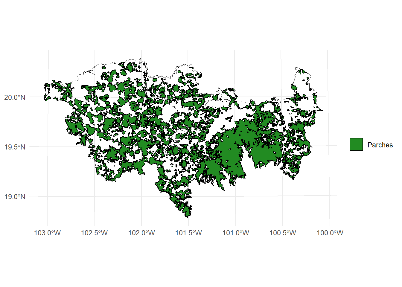

set.seed(10) #Para que seleccionen los mismos parches que yo

#Seleccionar de forma aleatoria a 100 de estos parches para restaurar
parches_restauracion <- sample(1:nrow(habitat_nodes), 100)

parches_restauracion
#>   [1] 137 330 368  72 211 344 271 143 403  24  13 351 392
#>  [14] 110 263 231 155 342 338 285 385 377  92  50 365 154
#>  [27] 101  33 135 379 158 324  93 114  88 307 182 242 288
#>  [40] 267 335 382 347  42 334 394 217 200 144  26 345 209
#>  [53]  48 151  15 395 317 132 227 270  35 266  74  58 167
#>  [66] 398  31 378 337 109  39 118  89  18 361 254 192 249
#>  [79]  90 234 251 328   4  63  20 321 224 241 176  94 148
#>  [92] 402 346  27  80 404 207 298 119 401

Creamos un nuevo campo llamado restauracion (puede ser cualquier nombre) con valores de 1 que representan parches que existen en el paisaje:

habitat_nodes$restauracion <- 1

Asignamos un valor de 0 a los parches seleccionados para restaurar (no existen en el paisaje inicialmente y serán restaurados.

habitat_nodes$restauracion[parches_restauracion] <- 0

Aplicamos la función MK_dPCIIC(). En este ejemplo usaremos el índice PC y una probabbilidad de 0.5 bajo un umbral de distancia de 10 km.

PCrestauracion <- MK_dPCIIC(nodes = habitat_nodes,
                attribute = NULL,
                area_unit = "ha",
                distance = list(type = "edge", keep = 0.1),
                LA = NULL,
                restoration = "restauracion",
                onlyrestor = TRUE,
                metric = "PC",
                probability = 0.5,
                distance_thresholds = 10000,
                intern = TRUE) #10 km
#> Estimating PC index. This may take several minutes depending on the number of nodes
#> 
  |                                                        
  |                                                  |   0%
  |                                                        
  |==================================================| 100%
#>  ■■■■■■■■■■■                       35% |  ETA:  3s
#> 
#> Done!
PCrestauracion
#> Simple feature collection with 404 features and 3 fields
#> Geometry type: POLYGON
#> Dimension:     XY
#> Bounding box:  xmin: -108954 ymin: 2025032 xmax: 202330.2 ymax: 2198936
#> Projected CRS: NAD_1927_Albers
#> First 10 features:
#>    Id restauracion    dPCres                       geometry
#> 1   1            1   0.00000 POLYGON ((54911.05 2035815,...
#> 2   2            1   0.00000 POLYGON ((44591.28 2042209,...
#> 3   3            1   0.00000 POLYGON ((46491.11 2042467,...
#> 4   4            0 -36.02491 POLYGON ((54944.49 2048163,...
#> 5   5            1   0.00000 POLYGON ((80094.28 2064140,...
#> 6   6            1   0.00000 POLYGON ((69205.24 2066394,...
#> 7   7            1   0.00000 POLYGON ((68554.2 2066632, ...
#> 8   8            1   0.00000 POLYGON ((69995.53 2066880,...
#> 9   9            1   0.00000 POLYGON ((79368.68 2067324,...
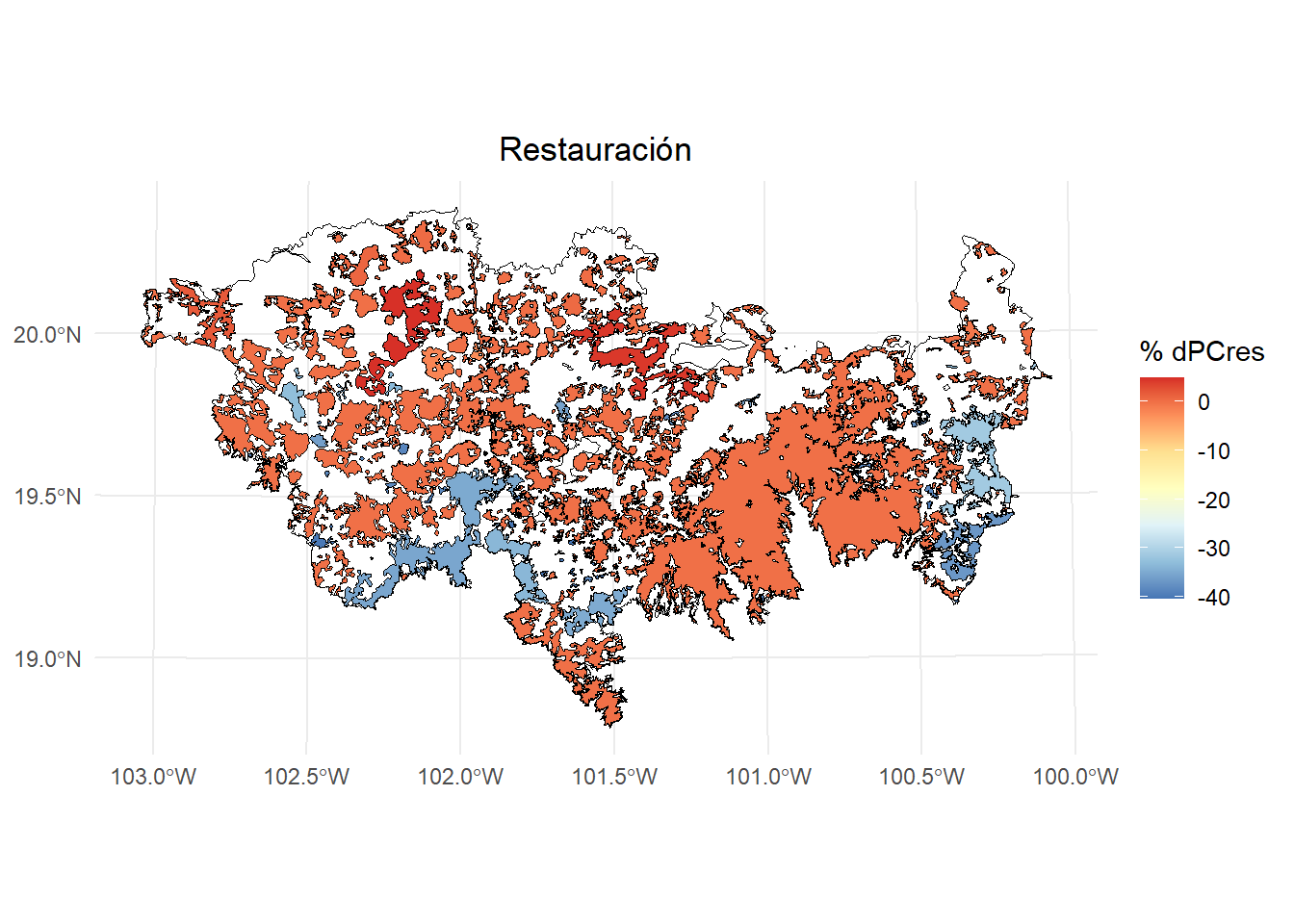
#> 10 10            1   0.00000 POLYGON ((23378.32 2067554,...

Se crea la columna dPCres con la importancia relativa del parche para mejorar la conectividad del paisaje al aparecer cuando es restaurado. Los valores van de -100 a 100, debido a que su contribución puede incluso ser negativa, es decir, disminuye la conectividad global al restaurarlo.

ggplot() +  
  geom_sf(data = paisaje, aes(color = "Study area"), fill = NA, color = "black") +
  geom_sf(data = PCrestauracion, aes(fill = dPCres), color = "black", size = 0.1) +
  scale_fill_distiller(
    palette = "RdYlBu",
    direction = -1, 
    name = "% dPCres"
  ) +
  theme_minimal() +
  labs(
    title = "Restauración",
    fill = "% dPCres"
  ) +
  theme(
    legend.position = "right",
    plot.title = element_text(hjust = 0.5)
  )

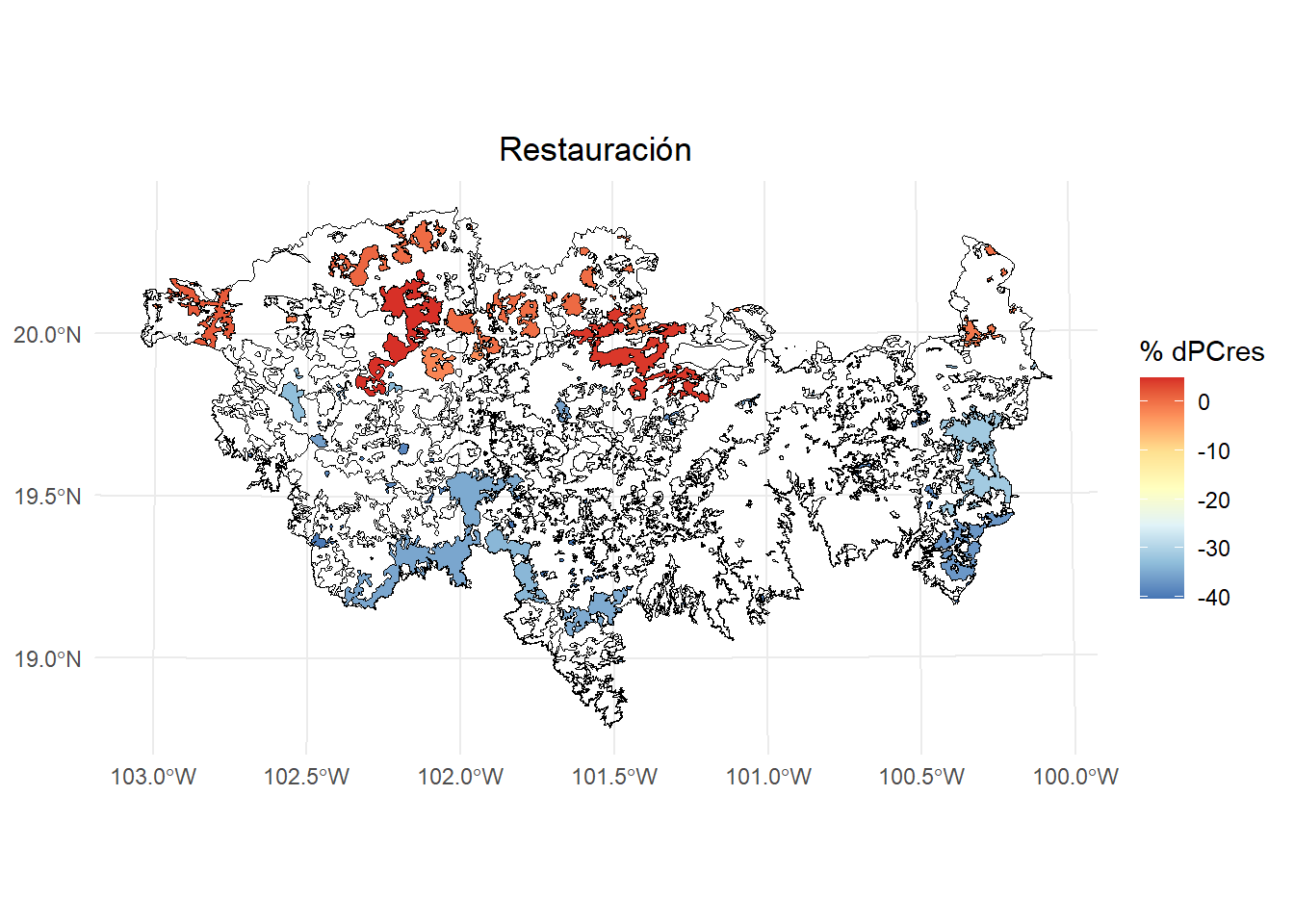
Veamos solo los parches de restauración


PCrestauracion2 <- PCrestauracion[PCrestauracion$restauracion == 0,]

ggplot() +  
  geom_sf(data = paisaje, aes(color = "Study area"), fill = NA, color = "black") +
  geom_sf(data = habitat_nodes, aes(color = "Patches"), fill = NA, color = "black") +
  geom_sf(data = PCrestauracion2, aes(fill = dPCres), color = "black", size = 0.1) +
  scale_fill_distiller(
    palette = "RdYlBu",
    direction = -1, 
    name = "% dPCres"
  ) +
  theme_minimal() +
  labs(
    title = "Restauración",
    fill = "% dPCres"
  ) +
  theme(
    legend.position = "right",
    plot.title = element_text(hjust = 0.5)
  )

Si desactivamos onlyrestor entonces estima los otros valores delíndice de conectividad (i.e., dPC, intra, flux y connector).

PCrestauracion <- MK_dPCIIC(nodes = habitat_nodes,
                attribute = NULL,
                area_unit = "ha",
                distance = list(type = "edge", keep = 0.1),
                LA = NULL,
                restoration = "restauracion",
                onlyrestor = FALSE,
                metric = "PC",
                probability = 0.5,
                distance_thresholds = 10000,
                intern = FALSE) #10 km
PCrestauracion
#> Simple feature collection with 404 features and 7 fields
#> Geometry type: POLYGON
#> Dimension:     XY
#> Bounding box:  xmin: -108954 ymin: 2025032 xmax: 202330.2 ymax: 2198936
#> Projected CRS: NAD_1927_Albers
#> First 10 features:
#>    Id restauracion       dPC  dPCintra   dPCflux
#> 1   1            1 0.0128564 0.0000006 0.0128558
#> 2   2            1 0.0332059 0.0000037 0.0332022
#> 3   3            1 1.6831849 0.0093299 1.6665804
#> 4   4            0 0.0184037 0.0000011 0.0184026
#> 5   5            1 0.0285162 0.0000026 0.0285136
#> 6   6            1 0.0040938 0.0000001 0.0040937
#> 7   7            1 0.0069481 0.0000001 0.0068704
#> 8   8            1 0.0088543 0.0000003 0.0088540
#> 9   9            1 0.0369150 0.0000032 0.0331109
#> 10 10            1 5.5556530 0.0665892 4.4246468
#>    dPCconnector    dPCres                       geometry
#> 1  0.000000e+00   0.00000 POLYGON ((54911.05 2035815,...
#> 2  0.000000e+00   0.00000 POLYGON ((44591.28 2042209,...
#> 3  7.274621e-03   0.00000 POLYGON ((46491.11 2042467,...
#> 4  0.000000e+00 -36.02491 POLYGON ((54944.49 2048163,...
#> 5  0.000000e+00   0.00000 POLYGON ((80094.28 2064140,...
#> 6  5.309968e-08   0.00000 POLYGON ((69205.24 2066394,...
#> 7  7.758334e-05   0.00000 POLYGON ((68554.2 2066632, ...
#> 8  0.000000e+00   0.00000 POLYGON ((69995.53 2066880,...
#> 9  3.800919e-03   0.00000 POLYGON ((79368.68 2067324,...
#> 10 1.064417e+00   0.00000 POLYGON ((23378.32 2067554,...

5 índice integral de conectividad y Probabilidad de conectividad

7 Prioridades de conservación y restauración con MK_Focal_nodes()